rkm0959

이어서 간다. 이번 글에서 다룰 주제는

• OSPEP를 이용한 DRS의 tight contraction factor
• OSPEP를 이용한 optimal parameter selection
• CVXPY를 이용한 위 주제들과 관련된 구현 몇 가지

Part 3. Tight Analytic Contraction Factors for DRS

결과부터 소개한다. 우리가 앞에서 준비했던, 논문의 정리 4.1.만 소개한다. 그래도 논문 링크를 열고 정리 4.1.~4.4.를 한 번 확인하는 것을 추천.

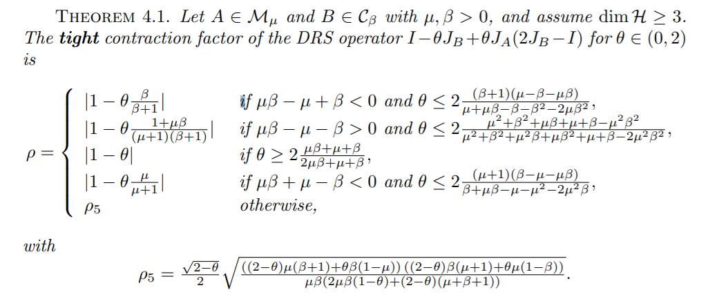
결과도 매우 중요하지만, 아무래도 일단 관심이 가는 것은 대체 이렇게 복잡한 것을 어떻게 증명했냐는 것이다. 논문의 말을 옮기면,

• 기본적으로 Mathematica 같은 Computer Algebra System은 필요하다
• OSPEP에서 얻은 Primal/Dual Problem을 활용한다. 이들을 풀기 위해서, 다음과 같은 접근을 사용한다.
• Primal : 핵심 아이디어는 worst-case operator가 $\mathbb{R}^2$ 위에서 존재할 것이라는 추측이다. 이는 Primal Problem의 해 $G^{*}$의 rank가 2 이하라는 것과 동치인데, 이 추측의 근거는 complementary slackness라고 한다. 이러한 2차원 위에서의 worst-case analysis는 SDP 대신 non-convex quadratic programming 문제로 분석할 수 있고, 이 문제에 대응되는 Karush–Kuhn–Tucker condition을 이용하여 문제를 해결했다고 한다.
• Dual : 역시 여기서도 Dual Problem의 해로 얻어지는 행렬 $S^{*}$가 rank 2 이하라는 가정을 한다. 근거는 Primal과 동일하다. 이 가정으로 $\rho^2$과 $\lambda_\mu^A$, $\lambda_\beta^B$ 사이의 관계식을 추가적으로 얻고, 이를 constraint로 하여 $\rho^2$을 최소화했다고 한다. 말이 쉽지만 정말 어려워 보인다..
• 이렇게 Primal/Dual 문제를 (analytical) 푼 다음, 그 결과가 같음을 확인하면 자동으로 증명이 끝난다.

Appendix를 구경하면 이 결과의 엄밀한 증명을 직접 볼 수 있다. ㄹㅇ 가슴이 웅장해진다... 

Part 4 : Optimal Parameter Selection with OSPEP

여기서는 operator class $\mathcal{Q}_1$, $\mathcal{Q}_2$를 알고 있을 때 parameter $\alpha, \theta$를 optimal 하게 설정하는 방법을 다룬다.

이는 결국 $\rho^2_{*} (\alpha, \theta)$를 해당 $\alpha, \theta$에 대한 optimal contraction factor라고 할 때, $$\rho^2_{*} = \inf_{\alpha, \theta > 0} \rho^2_{*}(\alpha, \theta)$$와 대응되는 $\alpha_{*}$, $\theta_{*}$를 찾는 문제와 같다. 원래 $\theta \in (0, 2)$라는 조건이 있으나, 이 조건은 relax 해도 무방하다. 

$\rho^2_{*}(\alpha, \theta)$의 값 자체는 SDP를 풀어서 계산할 수 있으니, 이차원 위에서 미분 불가능한 함수를 최소화하는 일반적인 알고리즘이 있다면 이를 사용하여 문제를 해결할 수도 있을 것이다. 그러나, 조금 더 작업을 거치면 더욱 편하게 문제를 풀 수 있다. $\theta$를 최적화 문제 안에 집어넣자.

Dual Problem $$\begin{equation*} \begin{aligned} \text{minimize} \quad & \rho^2 \\ \text{subject to} \quad & \lambda_\mu^A, \lambda_\beta^B \ge 0 \\ \quad & S = -M_O - \lambda_\mu^A M_\mu^A - \lambda_\beta^B M_{\beta}^B + \rho^2 M_I \succeq 0 \end{aligned} \end{equation*}$$을 다시 생각해보자. 우리가 $\alpha, \theta$를 고정된 값이 아니라 최적화 문제의 변수로 두지 못하는 이유는, 행렬 $S$의 entry가 $\alpha, \theta$의 nonlinear term을 포함하고 있기 때문이다. $\alpha$는 아예 분모에 있고, $\theta$는 $\theta^2$ 항이 $S$에 있다. 여기서 $\theta$에 대한 quadratic term을 제거하기 위해, Schur Complement를 사용한다.

$$\begin{equation*} \begin{aligned} S &= -M_O - \lambda_\mu^A M_\mu^A - \lambda_\beta^B M_{\beta}^B + \rho^2 M_I \\ S' &= - \lambda_\mu^A M_\mu^A - \lambda_\beta^B M_{\beta}^B + \rho^2 M_I \end{aligned} \end{equation*} $$라고 정의하면, $$M_O = (1, \theta, -\theta)^T (1, \theta, -\theta)$$이므로, Schur Complement의 성질에서 $S \succeq 0$는 $v = (1, \theta, -\theta)^T$라 했을 때 $$\overline{S} = \left[ \begin{matrix} S' & v \\ v^T & 1 \end{matrix} \right] \succeq 0$$과 동치이다. 또한, $S'$은 각 entry에 $\theta$에 대한 non-linear term이 없으므로, $\theta$까지 SDP에 넣을 수 있다.

즉, 새로운 문제를 $$\begin{equation*} \begin{aligned} \text{minimize} \quad & \rho^2 \\ \text{subject to} \quad & \lambda_\mu^A, \lambda_\beta^B, \theta \ge 0 \\ \quad & S' = - \lambda_\mu^A M_\mu^A - \lambda_\beta^B M_{\beta}^B + \rho^2 M_I \\ \quad & v = (1, \theta, -\theta)^T \\ \quad & \overline{S} = \left[ \begin{matrix} S' & v \\ v^T & 1 \end{matrix} \right] \succeq 0 \end{aligned} \end{equation*}$$로 바꾸면, $\theta$에 대한 최적화까지 자동으로 된다. 이제 남은 것은 $\alpha$에 대한 최적화다.

이렇게 해서 얻은 주어진 $\alpha$에 대한 optimal contraction factor를 $\rho^2_{*}(\alpha)$라고 하자. 이를 최소화하면 된다.

변수 하나에 대한 (미분 불가능한) 함수의 minimization은 다양한 방법이 있다. 그런데, 실험 결과에 따르면

•  함수 $\rho^2_{*}(\alpha)$는 연속함수이다. (별로 놀랍지는 않은 사실)
• 함수 $\rho^2_{*}(\alpha)$는 unimodal 함수이다. (놀라운 사실)

그러므로, 이를 최소화하기 위해서 (PS를 했던 사람의 입장에서 쉽게 생각하면) 삼분탐색을 사용해도 좋다.

사실 scipy나 matlab 등에서 이미 derivative-free optimization이 구현이 되어있기 때문에, 이걸 가져다 쓰면 된다.

Part 5 : Programming OSPEP with CVXPY

이건 논문에는 없고 (정확하게는 CVXPY로 하지 않고 MATLAB 등으로 한 것 같다) 그냥 내가 심심해서 하는 것이다.

논문의 저자들이 사용한 코드를 보고 싶다면, github.com/AdrienTaylor/OperatorSplittingPerformanceEstimation로 가자. 

내가 여기서 짠 코드들은 github.com/rkm0959/rkm0959_implements에 가면 있다. 

Task 1 : Verifying Theorem 4.1. Numerically

CVXPY를 이용하여 Theorem 4.1.을 검증해보자. 방법은 다음과 같다.

• $\alpha, \theta, \mu, \beta$를 적당히 랜덤하게 선정한다.  
• 대응되는 Primal/Dual Problem을 CVXPY로 해결한다. SDP를 풀어야하니, blas+lapack을 설치해야 한다.
• 또한, Theorem 4.1.을 이용하여 optimal contraction factor를 계산한다. 
• Theorem 4.1.에는 Case가 총 5가지가 있다. 이때, 어떤 Case에서 계산이 되었는지도 기록한다.
• Primal Problem, Dual Problem, Theorem 4.1.로 얻은 답이 일치하는지 확인한다.
• 위 과정을 여러 번 반복한 후, 5가지의 Case를 각각 몇 번 다루었는지를 확인한다.

이를 구현한 코드는 다음과 같다. 

이렇게 하여 Theorem 4.1.의 결과를 검수할 수 있다. SDP solver가 문제를 잘 해결할 수 있도록 극단적인 값들은 넣지 않았다.

각 코드의 의미는 거의 자명하니 (식을 그대로 옮긴 것에 불과하다) 자세한 설명은 생략하도록 하겠다. Task 1은 이렇게 끝.

Task 2 : Optimal Parameter Selection with OSPEP

이번에는 Part 4에서 다루었던 내용을 구현해보자. 우리가 할 일은

• 주어진 $\mu, \beta$에 대하여 optimal parameter $\alpha, \theta$를 계산
• $\rho^2_{*} (\alpha)$의 그래프를 그리고, 실제로 unimodal function인지 눈으로 확인
• 물론, 이러한 내용 및 그래프는 논문에도 있으며, DRS가 아니라 DYS로 설명되어 있다.

Part 4의 내용을 그대로 CVXPY로 옮기면, 다음과 같은 코드를 얻을 수 있다.

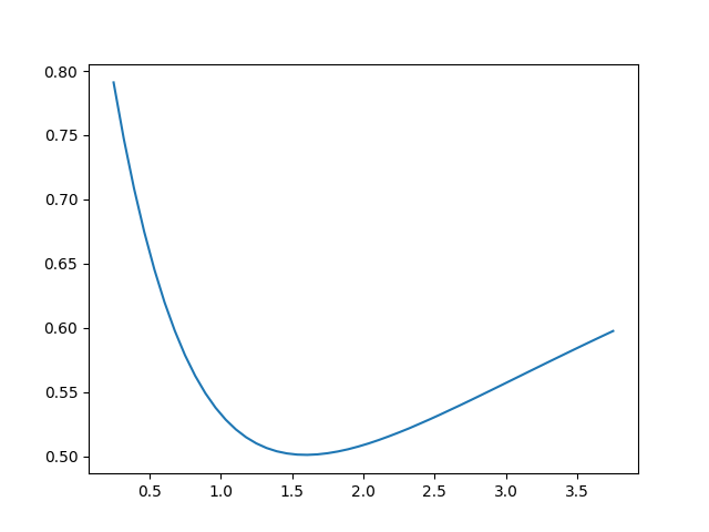
여기서 얻는 결론은 $\mu = 0.53$, $\beta = 1.35$일 때, optimal parameter는 $$\alpha_{*} = 1.5949751, \quad \theta_{*} = 1.4244099$$이고, 이때 얻어지는 optimal contraction factor는 $$\rho_{*} = 0.5010598$$이라는 것이다. 또한, 이 경우에 대한 $\rho^2_{*} (\alpha)$의 그래프를 그려서 unimodal function임을 확인할 수 있다. 그래프는 아래와 같다.

당연하지만, $x$축은 $\alpha$의 값, $y$축은 $\rho^2_{*}(\alpha)$의 값이다. 이렇게 Task 2와 논문 정리도 끝 :)

이제 본격적으로 논문을 읽어보자. 논문에서는 예시 문제를 Davis-Yin Splitting (DYS)로 두고 문제를 해결한다.

하지만 이 글에서는 예시 문제를 Douglas-Rachford Splitting (DRS)로 두고 해결하고자 한다. 이유는

• 일단 나도 손계산 연습을 해보고 싶고, operator가 3개인 DYS보다는 2개인 DRS가 간단함
• 앞선 글에서 DRS를 어느 정도 설명했으니 독자가 이해하기도 편할 것
• 이 논문의 Theorem 4에서 DRS에 대한 정리를 하는데, 직접 코드를 짜서 verify 해보고 싶음
• 그리고 솔직히 논문 내용 그대로 옮기면 재미없음 ㄹㅇㅋㅋ 대신 흐름은 그대로 유지할 것

이번 글에서는 다음 주제를 다룬다.

• Operator Splitting Performance Estimation Problem을 SDP로 변환하는 방법
• OSPEP로 얻어진 SDP의 Dual Problem과 그 의미 및 활용법

Part 1 : Operator Splitting Performance Estimation Problem to SDP

먼저 DRS를 다시 볼 필요가 있다. 우리는 $R_{\alpha A}R_{\alpha B}$가 nonexpansive operator이므로, 이를 $I$와 함께 섞어서 $$\frac{1}{2} I + \frac{1}{2} R_{\alpha A} R_{\alpha B}$$로 fixed point iteration을 돌렸다. 하지만 굳이 이렇게 섞을 필요는 당연히 없고, $\theta \in (0, 2)$에 대하여 $$\frac{2 - \theta}{2} I + \frac{\theta}{2} R_{\alpha A} R_{\alpha B}$$로 섞어도 된다. 여기에 $R_{\alpha A} = 2J_{\alpha A} - I$, $R_{\alpha B} = 2J_{\alpha B} - I$를 대입하면 $$I - \theta J_{\alpha B} + \theta J_{\alpha A} (2J_{\alpha B} - I)$$를 우리의 operator로 얻는다. 이제 목표는 이 operator가 "얼마나 contractive"한지 파악하는 것이다.

우리는 Performance Estimation Problem의 작은 문제에서 $\mathcal{F}_{\mu ,L}$에서 문제를 생각했다.

이번에 다루어 볼 operator class를 알아보자. 앞에서 정의한 네 가지 operator class들과 이들의 교집합을 생각한다.

• maximal monotone operator의 집합 $\mathcal{M}$
• $\mu$-strongly monotone이면서 maximal monotone인 operator의 집합 $\mathcal{M}_\mu$
• $L$-Lipschitz operator의 집합 $\mathcal{L}_L$
• $\beta$-cocoercive operator의 집합 $\mathcal{C}_{\beta}$

이제 본격적으로 문제를 서술할 준비가 되었다. $\mathcal{Q}_1, \mathcal{Q}_2$가 각각 operator class고, (단, 이들은 $\mathcal{M}$의 subset) $$T(z ; A, B, \alpha, \theta) = I - \theta J_{\alpha B} + \theta J_{\alpha A} (2J_{\alpha B} - I)$$이라 하자. 우리가 풀고자 하는 최적화 문제는, 고정된 $\alpha, \theta > 0$에 대하여, $$\begin{equation*} \begin{aligned} \text{maximize} \quad & \frac{ ||T(z;A,B,\alpha, \theta) - T(z';A,B,\alpha,\theta)||^2}{||z-z'||^2} \\ \text{subject to} \quad & A \in \mathcal{Q}_1, B \in \mathcal{Q}_2, z \neq z' \end{aligned} \end{equation*}$$이다. 즉, 최악의 경우에서도 $T$를 $L$-Lipschitz라고 부를 수 있는 가장 최적의 $L$을 구하는 것이다.

이제 문제를 조금씩 변형해가며 SDP로 만들어보자. Performance Estimation Problem과 크게 다르지 않다.

Step 1 : $T(z; A, B, \alpha, \theta)$를 표현하기 위해서, 다음과 같이 변수를 설정한다. $$z_B = J_{\alpha B} z, \quad z_A = J_{\alpha A}(2z_B - z), \quad T(z;A,B,\alpha, \theta) = z - \theta (z_B - z_A)$$

Step 2 : 분모에 있는 $||z-z'||^2$가 불편하다. 이를 일반성을 잃지 않고 $1$로 강제하고 싶은 마음이 자연스럽다.

다행히도 이는 가능하다. Operator class $\mathcal{Q}$가 임의의 $\gamma > 0$에 대하여 $$A \in \mathcal{Q} \iff (\gamma^{-1}I)A(\gamma I) \in \mathcal{Q}$$라면 $\mathcal{Q}$를 homogeneous 하다고 한다. 우리가 다루는 operator class는 전부 homogeneous.

이제 $\gamma = ||z-z'||$라고 하면, $z$들을 전부 $\gamma^{-1}z$로 교체하고 $A, B$를 $(\gamma^{-1} I)A(\gamma I)$, $(\gamma^{-1} I)B(\gamma I)$로 교체하자.

이래도 문제 없음은 homogeneous 성질에서 나온다. 또한, Step 1에서 얻은 식 정리를 그대로 사용해도 괜찮다는 것을 열심히 계산하면 알 수 있다.

결국 $||z-z'||=1$인 경우에서만 문제를 해결해도 무방하다는 사실을 얻는다. 제약 조건을 하나 추가하고, 분모를 날리자.

중간 점검을 하자면, 결국 우리가 풀 문제는 $$\begin{equation*} \begin{aligned} \text{maximize} \quad & ||z - \theta (z_B - z_A) - z' + \theta(z'_B - z'_A)||^2 \\ \text{subject to} \quad & A \in \mathcal{Q}_1, B \in \mathcal{Q}_2, ||z-z'||^2 = 1 \\ \quad & z_B = J_{\alpha B} z, z_A = J_{\alpha A}(2z_B - z) \\ \quad & z'_B = J_{\alpha B} z', z'_A = J_{\alpha A}(2z'_B- z') \end{aligned} \end{equation*}$$

Step 3 : 이제 슬슬 operator class $\mathcal{Q}$가 눈에 거슬린다. Interpolation의 아이디어를 적용하면 좋겠다.

뒤에서 Interpolation을 적용할 때 알게 되겠지만, 필요한 것은 두 점에 대한 Interpolation 조건이다.

즉, Graph에 $(x_1, q_1), (x_2, q_2)$가 속하는 operator $T \in \mathcal{Q}$가 존재할 조건만이 필요하다. 결론을 제시하면,

• $\mathcal{M}$ : $\langle q_1 - q_2, x_1 - x_2 \rangle \ge 0$
• $\mathcal{M}_\mu$ : $\langle q_1 - q_2 , x_1 - x_2 \rangle \ge \mu ||x_1 - x_2||^2$
• $\mathcal{C}_{\beta}$ : $\langle q_1 - q_2, x_1 - x_2 \rangle \ge \beta || q_1 - q_2||^2$
• $\mathcal{L}_L$ : $||q_1- q_2||^2 \le L^2 ||x_1 - x_2||^2$
• 단, $L$-Lipschitz 조건을 넣고 싶다면 무조건 $\mathcal{M} \cap \mathcal{L}_L$ 형태로 operator class를 잡아야 한다
• $\mathcal{Q}$가 위 operator class의 교집합이라면, 단순히 대응되는 조건을 모두 가져오면 된다.
• 즉, 두 점이 operator class의 조건을 만족시키면 무조건 interpolation도 된다는 것이 결론. 점의 개수가 많아지면 성립하지 않는다.
• TMI : monotone operator는 일반적인 경우에서도 maximal monotone operator로 interpolate 할 수 있다 (Zorn's Lemma)

논문의 Theorem 4.1을 직접 검증해보기 위해서, 대응되는 세팅인 $\mathcal{Q}_1 = \mathcal{M}_\mu$, $\mathcal{Q}_2 = \mathcal{M} \cap \mathcal{C}_\beta$를 생각해보자.

• $B$가 지나야 하는 점은 $(z_B, (z-z_B)/\alpha)$와 $(z'_B, (z'-z'_B)/\alpha)$
• 그러니 얻는 식은 $\langle ((z-z')-(z_B - z'_B))/\alpha, z_B - z'_B \rangle \ge \beta ||((z-z')-(z_B - z'_B))/\alpha||^2$
• $A$가 지나야 하는 점은 $(z_A, (2z_B - z-z_A)/\alpha)$와 $(z'_A, (2z'_B-z'-z'_A)/\alpha)$
• 그러니 얻는 식은 $\langle (2(z_B - z'_B) - (z-z') - (z_A - z'_A))/\alpha, z_A- z'_A \rangle \ge \mu ||z_A - z'_A||^2$

추가적으로, $||z-z'||^2 = 1$이라는 조건도 가지고 있다. 눈치챘겠지만, $z-z'$, $z_A-z_A'$, $z_B - z'_B$과 같이 두 변수의 차로 식이 표현된다.

이를 치환하고 정리하면, 우리가 원하는 것은 결국 $$\begin{equation*} \begin{aligned} \text{maximize} \quad & ||z - \theta (z_B - z_A)||^2 \\ \text{subject to} \quad & ||z||^2=1 \\ \quad & \langle z-z_B, z_B \rangle \ge (\beta/\alpha) ||z-z_B||^2 \\ \quad & \langle 2z_B - z , z_A \rangle \ge (1+\alpha \mu)||z_A||^2 \end{aligned} \end{equation*}$$를 얻는다. 이제 SDP를 꺼낼 준비가 완료되었다. 마찬가지로 Gram Matrix $$G = \left[ \begin{matrix} \langle z, z \rangle & \langle z_A, z \rangle & \langle z_B, z \rangle \\ \langle z, z_A \rangle & \langle z_A, z_A \rangle & \langle z_B, z_A \rangle \\ \langle z, z_B \rangle & \langle z_A, z_B \rangle & \langle z_B, z_B \rangle \end{matrix} \right]$$를 꺼내자. 작업하고 있는 공간의 차원이 3 이상이라는 가정하에서, 우리가 아는 것은 $G$가 Positive Semidefinite이라는 사실 뿐이다.

이제 다음과 같이 행렬을 정의하자. $$ M_O = \left[ \begin{matrix} 1 & \theta & -\theta \\ \theta & \theta^2 & -\theta^2 \\ -\theta & -\theta^2 & \theta^2 \end{matrix} \right], \quad M_I = \left[ \begin{matrix} 1 & 0 & 0 \\ 0 & 0 & 0 \\ 0 & 0 & 0 \end{matrix} \right]$$ $$ M_\beta^B = \left[ \begin{matrix} -\beta/\alpha & 0 & \beta/\alpha + 1/2 \\ 0 & 0 & 0 \\ \beta/\alpha + 1/2 & 0 & -\beta/\alpha - 1 \end{matrix} \right], \quad M_\mu^A = \left[ \begin{matrix} 0 & -1/2 & 0 \\ -1/2 & -(1+\alpha \mu) & 1 \\ 0 & 1 & 0 \end{matrix} \right]$$ 그러면 최종적으로 우리가 원하는 SDP 형태를 얻는다. $$\begin{equation*} \begin{aligned} \text{maximize} \quad & Tr(M_OG) \\ \text{subject to} \quad & G \succeq 0, Tr(M_IG) = 1 \\ \quad & Tr(M_\mu^A G), Tr(M_\beta^BG) \ge 0 \end{aligned} \end{equation*}$$

특히, 이 SDP formulation의 해를 가지고 "worst case"에 대응되는 operator $A, B$를 복원할 수 있다.

$Tr(M_O G)$가 최대가 되는 경우의 $G$를 찾았다면, Gram Matrix의 성질을 이용하여 $z, z_A, z_B$를 복원한 다음 interpolate 하면 끝이다.

Part 2 : The Dual Problem and its Interpretations/Usage

이제 얻은 SDP의 dual problem을 생각해보자. 전형적인 계산을 하면 결국 $$\begin{equation*} \begin{aligned} \text{minimize} \quad & \rho^2 \\ \text{subject to} \quad & \lambda_\mu^A, \lambda_\beta^B \ge 0 \\ \quad & S = -M_O - \lambda_\mu^A M_\mu^A - \lambda_\beta^B M_{\beta}^B + \rho^2 M_I \succeq 0 \end{aligned} \end{equation*}$$를 얻는다. 또한, "웬만하면" (regularity condition) Strong Duality가 성립함은 Slater's Condition으로 보일 수 있다.

이는 논문의 정리 3.3.으로, 나름 전형적인 증명이고 테크니컬하므로 생략. 중요한 것은 이 Dual Problem을 어떻게 바라보느냐, 그리고 어떻게 써먹느냐다.

눈치를 챘겠지만, notation을 $M_{\mu}^A$, $M_{\beta}^B$로 둔 이유는 사실 이 행렬들, 정확하게는 이 행렬들과 관련된 trace에 대한 조건이 $A$의 $\mu$-strongly monotone, $B$의 $\beta$-cocoercivity를 encode 한 것이기 때문이다. 이와 같이 operator class에 $A, B$가 속하게 되면 이로부터 얻어지는 부등식들이 있고, 우리가 증명할 수 있는 것은 기본적으로 이러한 부등식들의 nonnegative combination이다. 이 생각을 이어가면 결국 얻을 수 있는 결론은

• dual variable $\lambda_\mu^A$, $\lambda_\beta^B$은 $A, B$에 대응되는 부등식들에 대한 가중치이다. (그러니 $0$ 이상이다)
• feasible point에서의 $\rho$ 값은 해당 가중치를 사용하였을 때 얻어지는 contraction factor이며, 이는 optimal 값에 대한 upper bound다.

즉, "가중치를 이렇게 넣었더니 contraction factor가 이렇게 나왔다"는 사실 "dual problem의 feasible point를 찾았다"와 같다.

강조하자면, Primal/Dual Problem의 직관적인 의미는 각각

• Primal : 변수로 들어가는 것은 "최악의 경우에 해당하는 operator", 얻어지는 것은 "이런 contraction factor는 기대할 수 없다"는 결론
• Dual : 변수로 들어가는 것은 "증명에 사용될 가중치", 얻어지는 것은 "이런 contraction factor는 얻어질 수 있다"는 결론
• 특히, Duality Gap이 "웬만하면" (Slater's Condition) 0이므로, 정말 아무런 걱정도 할 필요가 없음

이제 Dual Problem의 의미를 알았으니, 활용하는 법도 파악할 수가 있다.

• Contraction Factor에 대한 Upper Bound를 확보할 수 있다. 애초에 dual problem에서 항상 나오는 결론이다.
• Dual Problem을 풀면 "증명에 사용될 가중치"를 얻을 수 있다! 그러니 여러 parameter에 대해서 문제를 수치적으로 풀어보고, 이를 통해서 어떤 가중치가 사용되는지 확인한 후, 이에 대한 analytical 공식을 때려맞춘뒤 엄밀한 증명을 시작할 수 (정확하게는, 시도할 수) 있다.
• Convex Optimization에서 수렴성 증명 중 상당 부분은 정말 단순 계산인데, 그 계산각을 재는 게 어렵다. (후에 Acceleration을 다루면 Lyapunov Function에서 또 이 이야기가 나올 것이다) 부등식들을 섞어먹을 가중치를 선정하는 것도 난이도가 상당하다. Dual Problem은 여기서 도움을 준다.

글 3개에 걸쳐서 arxiv.org/pdf/1812.00146.pdf 논문을 간단하게 정리한다.

저번 글과 비슷한 제목과 비슷한 아이디어를 갖고 있으나, 그 context가 약간 다르다.

저번 글에서는 Gradient Descent라는 거의 모두가 아는 context가 있어서 설명이 쉬웠으나, 이번에는 약간 다르다. 

일단 Operator Splitting이 무엇인지를 알아야 context를 이해할 수 있다. 그러니 이번 글에서는 이를 빠르게 설명한다.

• Disclaimer : 사실 아래에서 $\mathbb{R}^n$으로 말하는 것은 Real Hilbert Space로 보는 것이 맞는 것으로 알고 있다. 굳이 $\mathbb{R}^n$으로 쓰는 이유는 내가 실해석도 모르고 함수해석도 모르고 여러모로 모르는 게 많기 때문. 올해 공부를 하면 어떻게 해결할 수 있지 않을까 기대중이다.
• 아래 내용의 대부분은 www.math.snu.ac.kr/~ernestryu/courses/optimization.html의 6, 7강에서 공부할 수 있다.

set-valued operator는 $\mathbb{R}^n$의 한 점을 $\mathbb{R}^n$의 subset으로 보내는 operator이다.

만약 set-valued operator의 값이 empty set이거나 크기가 1인 집합이라면, 이를 single-valued operator라고 한다.

Example (Subgradient) : $f : \mathbb{R}^n \rightarrow \mathbb{R} \cup \{\pm \infty\}$가 convex 함수이고 모든 $y \in \mathbb{R}^n$에 대하여 $$f(y) \ge f(x) + \langle g, y-x \rangle$$이 성립하면 $g$를 $f$의 subgradient at $x$라고 부르며, subgradient의 모음을 $\partial f(x)$라고 쓴다. 이는 set-valued operator.

• $0 \in \partial f(x)$라면 $x$가 $f$의 값을 최소화하며, 그 역도 성립한다. 
• $\partial (f+g)(x) \supseteq \partial f(x) + \partial g(x)$임은 자명. 단, 집합끼리의 덧셈은 Minkowski Sum.
• $\text{dom} f \cap \text{int } \text{dom} g \neq \emptyset$이면 $\partial (f+g)(x) = \partial f(x) + \partial g(x)$. 증명은 여기. 단 domain은 $f(x) < \infty$인 점들의 집합.

함수에 대하여 Convex, $L$-smooth, $\mu$-strongly convex 등을 정의하는 것을 operator에도 비슷하게 할 수 있다.

operator $A$가 있다. 각 $x, y \in \mathbb{R}^n$와 $u \in Ax$, $v \in Ay$에 대하여 ($A(x), A(y)$를 $Ax, Ay$라고 간단하게 표기한다)

• $\langle u-v, x-y \rangle \ge 0$이면, $A$를 monotone operator라 한다.
• $\langle u-v, x-y \rangle \ge \mu ||x-y||^2$이면, $A$를 $\mu$-strongly monotone operator라 한다.
• $\langle u-v, x-y \rangle \ge \beta||u-v||^2$이면, $A$를 $\beta$-cocoercive라 한다.
• $||u-v|| \le L||x-y||$라면 $A$를 $L$-Lipschitz라 한다. 물론, $\mu, \beta, L > 0$.
• 특히, $1$-Lipschitz인 operator를 nonexpansive operator라고 한다.

operator $A$에 대응되는 graph를 $\{(x, u) : u \in Ax\}$라고 정의하자.

또한, operator $A$가 다음 조건을 만족하면, $A$를 maximal monotone 하다고 정의한다.

• $A$는 monotone operator
• operator $B$가 다음 조건을 만족하면, $A = B$
• $B$는 monotone operator이며, $B$의 graph는 $A$의 graph를 포함한다.

operator $A$의 inverse를 $\{(u, x) : u \in Ax\}$를 graph로 갖는 operator라고 정의하자.

$A$의 resolvent operator를 $J_A = (I+A)^{-1}$로 정의한다. 물론, $I$는 identity operator이다.

또한, reflected resolvent operator를 $R_A = 2J_A - I$로 정의한다. resolvent는 뒤에서 중요한 역할을 한다.

최적화 문제와의 관련성을 본격적으로 논의해보자. 기본적으로, 다음과 같은 세팅을 거친다.

• 최적화 문제를 operator에 대한 문제로 바꾼다. 예를 들어, $f$의 최솟값을 구하는 문제는 $\partial f$의 zero를 찾는 문제가 된다.
• 이를 operator $T$의 fixed point를 찾는 문제로, 즉 $z \in Tz$인 $z$를 찾는 문제로 바꾼다. 이를 fixed point encoding이라고 부른다.
• operator $T$의 fixed point를 찾기 위해서, $z^{k+1} = Tz^k$를 반복한다. 이것이 수렴하면 성공이다.

operator $T$가 identity operator $I$와 nonexpansive operator $N$의 convex combination이라면 (단, $I$에 대응되는 비율이 nonzero) $T$를 averaged operator라고 부른다. 이 경우, $T$가 fixed point를 가진다면 $z^{k+1} = Tz^k$가 잘 수렴함을 증명할 수 있다. 증명 방식은 나중에 다루도록 하겠다.

특히, $T$가 $L$-Lipschitz고 $L<1$이라면, 수렴 속도가 기하급수적으로 빠르다는 것은 쉽게 증명할 수 있는 사실이다.

이제 fixed point encoding의 예시를 몇 개 보이는 것으로 이론적인 준비를 마치도록 하겠다.

Proximal Point Method : $A$가 maximal monotone이면 다음이 성립한다.

• $J_A$가 averaged operator : $R_A = 2J_A - I$가 nonexpansive 함을 쉽게 보일 수 있다. 특히, $J_A$는 single-valued.
• Minty Surjectivity Theorem : $J_A$의 domain은 $\mathbb{R}^n$이다. 즉, 모든 $x \in \mathbb{R}^n$에 대하여 $J_Ax$는 nonempty.

또한, $f$가 convex, closed, proper (CCP) function이라면, $\partial f$가 maximal monotone operator임을 보일 수 있다.

• Convex : $f(\theta x + (1-\theta)y) \le \theta f(x) + (1-\theta)f(y)$ for $\theta \in [0, 1]$
• Closed : $\{(x, \alpha) \in \mathbb{R}^n \times \mathbb{R} : f(x) \le \alpha\}$ is closed
• Proper : $f(x) \neq -\infty$ always, and $f(x) < \infty$ somewhere

이제 준비를 할 수 있다. $f$가 CCP function이라고 하면, 

• $f$의 최솟값을 구하는 문제를 $\partial f$의 zero를 찾는 문제로 바꿀 수 있다.
• 이를 $J_{\alpha \partial f} = (I + \alpha \partial f)^{-1}$의 fixed point를 찾는 문제로 바꿀 수 있다. 단, $\alpha > 0$.
• 그러니 $x^{k+1} = J_{\alpha \partial f}(x^k)$를 반복하여 문제를 해결할 수 있다. 이것이 Proximal Point Method.

Douglas-Rachford Splitting (DRS) : 이번에는 maximal monotone operator $A, B$가 있다고 가정하고, $$ 0 \in (A+B)x$$인 $x$를 찾는 문제를 생각하자. 열심히 계산하면, 이는 결국 $$x = J_{\alpha B}z, \quad R_{\alpha A}R_{\alpha B} z = z$$인 $(x, z)$를 찾는 문제와 같음을 알 수 있다. ($\alpha > 0$) 그러니 fixed point encoding을 얻는다.

그런데 $R_{\alpha A} R_{\alpha B}$는 nonexpansive 하지만 averaged operator는 아닐 수 있다. 그러므로, 이 문제를 해소하기 위하여 $$z^{k+1} = \left( \frac{1}{2} + \frac{1}{2} R_{\alpha A} R_{\alpha B} \right) z^k$$라고 하면 이는 averaged operator를 사용하였으니 수렴이 보장되는 fixed point iteration이 된다. 이를 통해서 문제를 해결할 수 있다.

이처럼 operator 여러 개가 섞인 문제를 쪼개서 푸는 것을 operator splitting이라고 한다.

예고 : 목표는 Operator Splitting Method에 대해서 Performance Estimation을 하는 것이다. 예를 들어, DRS에서는 iteration을 averaged operator $$ \frac{1}{2} I + \frac{1}{2} R_{\alpha A} R_{\alpha B}$$를 이용하여 했었다. $A, B$가 단순히 maximal monotone이 아니라 추가적인 성질을 가지고 있다면, 이 operator가 $L$-Lipschitz가 ($L<1$) 될 수도 있을 것이다. 이때, 우리가 보장할 수 있는 최선의 $L$ 값은 얼마일까? 그리고 이러한 문제를 어떻게 응용할 수 있을까? 다음 글에서 알아보도록 하자.

이 글에서는 논문 www.di.ens.fr/~ataylor/share/PESTO_CDC_2017.pdf를 정리한다.

(지금 보니까 저 논문은 toolkit 소개고, 아이디어 자체는 arxiv.org/pdf/1502.05666.pdf를 보는 게 더 좋을 것 같다)

보통 우리는 문제가 주어지면

• 이를 해결하는 알고리즘을 설계하고
• 최악의 경우에 어떻게 작동하는지 분석

한다. 만약 PS를 하는 사람이라면 답을 정확하게 구하는 알고리즘을 설계한 후, 최악의 경우의 시간복잡도를 분석할 것이다.

비슷하게, 최적화에서는 보통 답을 iterative 하게 근사하는 알고리즘을 설계한 후, 최악의 경우의 수렴성을 분석한다.

이 논문은 "최악의 경우의 수렴성"을 분석하는 자동화된 toolkit을 제시하는 논문이다. toolkit 링크는 여기다. Matlab으로 작성되어 있다.

toolkit의 기본 작동 원리를 알기 위해서, 작은 문제를 하나 풀어보자.

문제 (Informal) : $\mu$-strongly convex, $L$-smooth function $F$가 있다. $F$를 최소화하는 문제를 풀고자 한다. Initial point $x_0$에서 Gradient Descent를 적용하여 $x_1 = x_0 - \gamma \nabla F(x_0)$를 얻었을 때, $||\nabla F(x_1)||$의 크기를 얼마나 잘 줄일 수 있을까? 최악의 경우를 비교하여, 최선의 $\gamma$를 구할 수 있을까?

• $\mu$-strongly convex, $L$-smooth의 의미는 이 글과 이 글에서 매우 잘 정리되어 있다. 
• $\mu$-strongly convex, $L$-smooth function의 집합을 $\mathcal{F}_{\mu, L}$이라고 쓴다.

이 문제를 엄밀하게 서술하려면, 이를 최적화 문제 형태로 서술해야 한다. $$\begin{equation*} \begin{aligned} \text{maximize}  \quad  & ||\nabla F(x_1)||^2 \\  \text{subject to} \quad & F \in \mathcal{F}_{\mu, L} \\ \quad & x_1 = x_0 - \gamma \nabla F(x_0) \end{aligned} \end{equation*}$$ 그런데 이렇게만 쓰면 답이 $\infty$인 것이 뻔하므로, 추가적인 제약조건이 필요하다. 예를 들어, $|| \nabla F(x_0) ||^2$의 크기에 제약조건을 걸 수 있다. 그러면 $$\begin{equation*} \begin{aligned} \text{maximize}  \quad  & ||\nabla F(x_1)||^2 \\  \text{subject to} \quad & F \in \mathcal{F}_{\mu, L} \\ \quad & x_1 = x_0 - \gamma \nabla F(x_0) \\ \quad & ||\nabla F(x_0)||^2 \le R^2 \end{aligned} \end{equation*}$$ 라는 최적화 문제를 얻는다. 그런데 $F \in \mathcal{F}_{\mu, L}$가 변수라는 점이 문제 해결을 어렵게 한다. 

여기서 멋진 아이디어가 사용된다. 먼저, 우리가 $F$라는 함수에 접근하는 점은 $x_0, x_1$ 두 곳이다. 

그러니 사실 우리는 $f_i = F(x_i)$, $g_i = \nabla F(x_i)$의 값에만 관심을 가져도 충분하다. 이제 최적화 문제를 쓰면 $$\begin{equation*} \begin{aligned} \text{maximize}  \quad  & ||g_1||^2 \\ \text{subject to} \quad & \exists F \in \mathcal{F}_{\mu, L} \text{  s.t.  } F(x_i) = f_i, \nabla F(x_i) = g_i \\ \quad & x_1 = x_0 - \gamma g_0, \text{  } ||g_0||^2 \le R^2 \end{aligned} \end{equation*}$$의 형태가 된다. 그러니, 우리가 관심을 갖게 되는 문제는

• 언제 $F(x_i) = f_i$, $\nabla F(x_i) = g_i$를 만족하는 $F \in \mathcal{F}_{\mu, L}$이 존재할까?

가 된다. 이런 문제는 Lagrange Interpolation의 향기가 나고, 실제로 Interpolation이라고 불린다. 

그리고 $F \in \mathcal{F}_{\mu, L}$로 interpolation이 되는 조건은 이 논문에서 이미 증명이 되었다.

결론은 각 $i \neq j$에 대하여 부등식 $$f_i \ge f_j + \langle g_j, x_i - x_j \rangle + \frac{1}{2(1-\mu / L)} \left( \frac{1}{L} ||g_i - g_j||^2 + \mu ||x_i - x_j||^2  - 2 \frac{\mu}{L} \langle g_j - g_i, x_j - x_i \rangle \right)$$이 성립하는 것이, 원하는 interpolation 조건을 만족하는 $F \in \mathcal{F}_{\mu, L}$이 존재할 필요충분조건이라는 것이다.

이제 최적화 문제의 constraint 첫 줄을 interpolation 조건으로 교체할 수 있다. 또한, $x_1 = x_0 - \gamma g_0$를 대입하여 $x_1$ 변수를 제거할 수 있다.

남은 문제를 바라보면 다루고 있는 변수가

• $f_0$, $f_1$ : 이 값들은 constraint에서 그냥 혼자 있는 값들이다.
• $g_0, g_1, x_0$ : 이 값들은 objective나 constraint나 무조건 다른 값과 내적이 되어있다. 

이 성질 때문에, 문제를 Semidefinite Programming (SDP) 형태로 바꿀 수 있다. Gram Matrix $$G = \left[ \begin{matrix} \langle x_0, x_0 \rangle & \langle g_0, x_0 \rangle & \langle g_1, x_0 \rangle \\ \langle x_0, g_0 \rangle & \langle g_0, g_0 \rangle & \langle g_1, g_0 \rangle \\ \langle x_0, g_1 \rangle & \langle g_0, g_1 \rangle & \langle g_1, g_1 \rangle \end{matrix} \right]$$를 생각하자. Gram Matrix의 성질에 의하여, 다음이 성립한다.

• $G$는 Positive Semidefinite이며, 특히 풀고 있는 문제가 $\mathbb{R}^d$ 위의 문제면 rank가 최대 $d$.
• Positive Semidefinite이며 rank가 최대 $d$인 행렬이 주어지면, 이를 Gram Matrix로 보고 vector $x_0, g_0, g_1$을 복원할 수 있음.

그러므로 우리의 모든 문제를 $f_0$, $f_1$과 $G$에 대한 문제로 볼 수 있으며, $G$에 대해 명시할 조건은 $G$가 Positive Semidefinite이라는 점과 rank가 $d$ 이하라는 점이다. 하지만 우리의 관심사는 일반적인 $d$에 대한 것이므로, rank 조건은 제거해도 무방하다. (당장 $d \ge 3$이기만 해도 rank 조건이 무의미하다)

이제 남은 문제를 보면 진짜 단순한 Semidefinite Programming 문제고, 이는 standard solver로 해결할 수 있다.

논문에 의하면, 이렇게 SDP로 문제를 변형하여 해결할 수 있는 경우는 다음을 포함한다.

• Class of Functions : Smooth Convex, Strongly Convex, Bounded Subgradients, Bounded Domains, Non-Convex Smooth 등
• Methods : First-Order Methods : Subgradient, Proximal Operator 등
• Performance Measure (objective 설정) : $||x_n - x_{*}||^2$, $||\nabla F(x_n)||^2$, $F(x_n) - F(x_{*})$ 등
• Initial Condition : Performance Measure와 동일함. 물론, $x_n$ 대신 initial point $x_0$에 대한 조건.

그리고 이 toolkit은 이러한 경우 대부분을 지원한다고 한다. 갖고 놀기 좋은 것 같은데, 아직 쓰는 법은 모른다 ㅎㅎ;

궁금한 점은 이 toolkit으로 답을 $\mu$, $L$에 대한 수식으로 얻으려면 수식이 변수로 들어가있는 Symbolic한 SDP를 해결해야 할텐데, 이건 대체 어떻게 한 건지 궁금하다. toolkit 보면 수식으로 답을 얻어주는 것 같은데... 관련 논문 읽어봐도 아이디어는 알겠으나 이 점이 계속 헷갈린다. 더 공부하는 걸로.

UPD : 직접 돌려본 결과, 수치적으로 계산해준다. 그냥 예시에 답이 이렇게 나와야 한다고 주석으로 써있는 것..

arxiv.org/pdf/1502.05666.pdf 논문의 추가적인 내용은

• Interpolation 관련 엄밀한 증명
• SDP로 문제를 변환하는 것과, 해당 문제의 성질에 대한 엄밀한 증명
• SDP로 변환된 문제의 Lagrangian Dual을 생각하여, Upper Bound를 계산
• 특히, Slater Condition을 이용하여 "웬만하면" Duality Gap이 없음을 증명
• Performance Estimation Problem의 여러 응용 : 이걸로 문제를 많이 해결/제시하는 것 같다

I participated in UnionCTF as a member of Super Guesser. We reached 1st place :)

Mordell Primes

Solution

The main intuition is that the numerator of $kP$ will grow very fast as $k$ increases. This can be verified by simply checking for small $k$.

Therefore, we can try to simply brute force the value of $k$ and see if the numerators multiply to $N$.

Human Server

Solution

We have to do a MITM attack, but there are some twists - Alice and Bob do a check later to see if they have the same shared secret.

Suppose Alice's secret key, public key is $d_1$, $d_1G$ and Bob's secret key, public key is $d_2$, $d_2G$.

Now let's forward Alice's key as $e_1G$ and give the nonce $r_1$ to Bob, where we know the value $e_1$.

This will make Bob's shared secret equal to $(e_1d_2G).x \oplus r_1$. Since $d_2G$ is a known value and $e_1, r_1$ are known, we can calculate this.

Similarly, let's forward Bob's key as $e_2G$ and give the nonce $r_2$ to Alice, where we know the value $e_2$.

This will make Alice's shared secret equal to $(e_2d_1G).x \oplus r_2$. We have to make this equal to Bob's shared secret. 

This can be done by selecting $r_2$ as $$r_2 = (e_1d_2G).x \oplus (e_2d_1G).x \oplus r_1$$ and we can pass the check between Alice and Bob. We now know the shared secret, so the challenge is solved.

Of course, we can just choose $e_1 = e_2 = 1$ and some random value for $r_1$.

Cr0wn St3rling

Solution

We start by making some quick observations -

• The length of key_indexes must be 8 due to the check is_valid_number.
• There are only $7^8$ keys since there are 7 possible choices for each entry of the musical key.
• Actually, the first entry of key_indexes is guaranteed to be 1. Make that $7^7$ valid key_indexes.
• Fibonacci function is implemented pretty badly, and we can change that to simple dynamic programming
• There's nothing we need to do about the $\pi$ function
• The q_grid function is suboptimal, but it runs in decent time so no need to worry about that.

We will now decrease the number of key_index candidates by using the known plaintext "union".

• Each entry of key_indexes works in a separable way, so we can work with each entry separately
• There are 7 possible choices for a specific key_indexes entry
• The problem is we do not know the length of q_grid (we do not know the variable $size$ in advance)
• For $i < 5$, the maximum value of the index is $7^4 \cdot 3$, which is small compared to the length of the q_grid for $size = 75000$.
• Therefore, we can reasonably assume that the length of q_grid is larger than the index.
• Now we can try out each candidate for a specific key_indexes entry - this is sufficient to get the first 5 entries of key_indexes.

We now have only $7^3$ candidates to work with. We can try every single one of them.

• The only slow part of the brute force is generating the q_grid and calculating its length.
• This can be done very fast by calculating q_grid for $size = 75000$ and using binary search to calculate the "actual length of the q_grid" (i.e. number of entries that are less than the actual "size" variable)
• However, since we have a lot of time, we can just calculate q_grid for $size = 75000$ then simply calculate the actual length of the q_grid with brute force. It doesn't take too long for us to get the flag anyway..

Neo-Classical Key Exchange

Solution

The first thing we notice is that list_valid checks if the length of the list is a square, and list_iter simply returns the square root.

Now we look at the main function, the list multiplication. If we stare at it for a while (and notice the "length is a square" stuff) we can find out that this list multiplication is just a matrix multiplication, where the list is the matrix entries in order.

Now we have to solve a Diffie-Hellman problem with matrices over $\mathbb{F}_p$. We will do it by solving discrete logarithm problem.

• Idea 1 : The range of the secret keys
• The range of the secret keys are from $2$ to $p$ - this implies that we do not need the entire discrete logarithm, just some part of it.
• Idea 2 : The determinant
• This idea can give us the required information of the (matrix) discrete logarithm if we calculate the respective discrete logarithm (over finite field $\mathbb{F}_p$) on the determinants. However, the primes used here are quite large, which makes this approach infeasible.

Instead of $5 \times 5$ matrices that we actually have to deal with, we first look at $2 \times 2$ matrices over the reals.

The idea is that we want to look at how matrix powers behave in a more relaxed setting, and find some properties we can use in $\mathbb{F}_p$.

We try to solve $A^k = B$. Take the Jordan Canonical Form $J$ with $A = PJP^{-1}$. Then we want to solve $$J^k = P^{-1}BP$$ so we may simply assume that $A$ is in a Jordan Canonical Form. If $A$ is in the form of $$A = \left[ \begin{matrix} \lambda_1 & 0 \\ 0 & \lambda_2 \end{matrix} \right]$$ then nothing special happens - we still need a logarithm to compute $k$, which is infeasible in $\mathbb{F}_p$. However, if $A$ is in the form of $$A = \left[ \begin{matrix} \lambda & 1 \\ 0 & \lambda \end{matrix} \right]$$ then we have some interesting phenomenon : $$A^k = \left[ \begin{matrix} \lambda^k & k \lambda^{k-1} \\ 0 & \lambda^k \end{matrix} \right]$$ and now we can get $k$ as $(k\lambda^{k-1} \times \lambda) / \lambda^k$, all of which we know and can be done in $\mathbb{F}_p$.

Let's come back to $\mathbb{F}_p$. If we want to use the Jordan Canoncial Form trick, we need our characteristic polynomial to completely split in $\mathbb{F}_p$, and we also need a block of size $2$. Our matrix satisfies all of these properties, so we can just use the exact same technique here as well.

Of course, we can see that we have calculated the discrete logarithm modulo $p$, not the full discrete logarithm.

However, because of Idea 1 (secret key range is small) this is enough to solve the problem. Here are some additional notes.

• The Jordan Canonical Form of our matrix $G$ has 4 blocks of size 1, 1, 1, 2. 
• This actually shows that the order of $G$ is $p(p-1)$ - this can be seen as the $p-1$ term dealing with the diagonal entries (Fermat's Theorem) and the $p$ term dealing with the off-diagonal term in our block of size 2. 
• If we want to solve for the discrete logarithm modulo $p-1$, we need discrete logarithm over $\mathbb{F}_p$ which we decided infeasible.
• I think there are some similarities with this challenge and TetCTF 2021 unevaluated.

Why is a raven

Solution

This is Supersingular Isogeny Diffie-Hellman protocol. Looking at the Wikipedia article and back, we see that we have extra information, $$\phi_A(P_A), \phi_A(Q_A)$$ Since $\phi_A$ has $S_A = P_A + k_AQ_A$ as it's kernel, we see that $$ \phi_A(P_A + k_AQ_A) = \phi_A(P_A) + k_A \phi_A(Q_A) = 0$$ Also, since the values here are in a subgroup of order $2^{216}$, we can calculate $k_A$ (i.e. discrete logarithm) efficiently with Pohlig-Hellman.

Now that we know $k_A$, one of the secret keys, we can just follow our algorithm to calculate the shared secret.

github.com/rkm0959/rkm0959_implements/tree/main/Chebyshev%20Acceleration

매우 최근에 올라온 Acceleration에 대한 Survey Paper arxiv.org/abs/2101.09545을 읽는다. 이 글은 2장을 정리한다.

일단은 관심가는 부분만 읽을 예정인데, 아마 3장을 제일 마지막에 읽을 것 같다. 사전지식이 부족한 경우 이 자료 참고.

Acceleration Survey Paper + OSPEP + Proximal Algorithms Survey Paper 이렇게 읽으면 지식이 좀 쌓이지 않을까 생각중이다..

모든 정리의 번호는 Survey Paper와 같은 번호를 사용한다. 단순히 정리 블로그니까 논문 표현을 그대로 가져다 쓰는 일도 많을 것이다.

이 글에서는 unconstrained quadratic minimization 문제, 즉 $f(x) = \frac{1}{2} x^T Hx - b^Tx$를 최소화하는 문제를 다룬다. 물론 $H$는 symmetric.

이 문제의 optimal point는 $x^{*} = H^{-1}b$임이 자명하다. 즉, 이 문제는 결국 linear system의 해를 빠르게 구하는 문제와 같다.

보통 이러한 minimization 문제를 만나면, 많은 사람들이 Gradient Descent를 생각할 것이다. 

즉, initial point $x_0$와 step-size $\gamma$를 잡고, $x_{i+1} = x_i - \gamma \nabla f(x_i)$를 반복하는 것이다.

이 식을 정리하면 $x_{i+1} = (I - \gamma H) x_i + \gamma b$를 얻고, $x^{*}$의 식을 이용하면 $$x_{k+1} - x^{*} = (I - \gamma H) (x_k - x^{*})$$를 얻는다. 이제 우리의 목표는 $I - \gamma H$의 matrix norm을 최소화하는 것이다. 우리는 일반적으로 2-norm, 즉 Spectral Norm을 생각한다.

이제 잠시 $H$로 가능한 행렬의 범위를 좁혀, 적당한 $\mu, L > 0$에 대해 $\mu I \le H \le L I$가 성립한다고 가정하자.

그러면 우리는 $\gamma$를 선택하는 과정에서 worst-case convergence를 최선으로 하기 위해서 $$\max_{\mu I \le H \le LI} ||I - \gamma H||_2$$를 최소화할 필요가 있다. 이 문제는 결국 $\text{max}(|1-\mu \gamma|, |L \gamma - 1|)$를 최소화하는 것이다. 그러니 $\displaystyle \gamma = \frac{2}{\mu + L}$를 잡을 수 있다.

특히 이 경우 $\displaystyle ||I - \gamma H||_2 \le \frac{L - \mu}{L + \mu} = \frac{\kappa - 1}{\kappa + 1}$이고 ($\kappa = L / \mu$는 condition number) $$||x_k - x^{*}||_2 \le \left( \frac{\kappa - 1}{\kappa + 1} \right)^{k} ||x_0 - x^{*}||_2$$를 얻는다. 이것이 Gradient Descent의 수렴 속도가 되겠다. 이를 더 빠르게 하는 것이 우리의 목표다.

이번에는 조금 더 넓은 class의 알고리즘을 생각해보자. $x_{k+1}$을 $x_k$에 $\nabla f(x_k)$의 상수배를 더한 것만 고려하지 말고, 아예 $$x_{k+1} \in x_0 + \text{span} \{ \nabla f(x_0), \cdots , \nabla f(x_k) \}$$를 고려하자. 이 경우, 단순한 수학적 귀납법으로 다음을 보일 수 있다.

Proposition 2.1. : 위와 같은 방식으로 $x_k$를 계산한 경우, 다항식 $P_k$가 있어 $\text{deg}(P_k) \le k$, $P_k(0) = 1$이고 $$x_k - x^{*} = P_k(H)(x_0 - x^{*})$$ 이제 우리는 앞선 사고방식을 그대로 따라가면 $$\displaystyle \max_{\mu I \le H \le LI} ||P_k(H)||_2$$를 최소화하고 상수항이 $1$인 $k$차 이하 다항식 $P_k$를 찾아야 한다. 그런데 $H$가 symmetric이므로, 이 문제는 사실 $$\max_{\mu \le \lambda \le L} |P_k(\lambda)|$$를 최소화하는 것과 같다. 이제 짬이 좀 찬 독자들은 Chebyshev라는 단어가 왜 나왔는지 알 것이다. 저런 문제에서 최적의 다항식이 Chebyshev Polynomial이기 때문이다. 이들은 $[-1, 1]$ 위에서 최적이기 때문에, $[\mu, L]$을 $[-1, 1]$로 shift 하는 처리 작업이 필요하다. 즉, $$t : x \rightarrow \frac{2x - (L + \mu)}{L - \mu}$$의 처리를 하자. 또한, $P_k(0)=1$이라는 조건이 있으니 이것도 처리해야 한다. 결과적으로 우리는 $$C_k^{[\mu, L]}(x) = \frac{T_k(t(x))}{T_k(t(0))}$$라는 다항식을 정의할 수 있다. 이제 목표는 $$x_k - x^{*} = C_k^{[\mu, L]}(H) (x_0 - x^{*})$$가 성립하도록 효율적인 iteration을 설계하는 것이다. 이를 위해서는 $C_k^{[\mu, L]}$에 대한 점화식이 필수적이다. 결과적으로, $$\delta_0 = -1, \quad \delta_k = \frac{L - \mu}{2(L + \mu) - \delta_{k-1}(L - \mu)}$$ $$C_0^{[\mu, L]}(x) = 1, \quad C_1^{[\mu, L]}(x) = 1 - \frac{2}{L + \mu}x, \quad C_k^{[\mu, L]}(x) = \frac{2\delta_k (L+\mu - 2x)}{L - \mu} C_{k-1}^{[\mu, L]}(x) + \left( 1 - \frac{2\delta_k (L+\mu)}{L - \mu} \right) C_{k-2}^{[\mu, L]}(x)$$가 성립함을 보일 수 있다. Chebyshev Polynomial의 점화식을 가지고 열심히 계산하면 될 것으로 예상한다.

이제 이를 $x_k - x^{*} = C_k^{[\mu, H]}(x_0 - x^{*})$에 집어넣고 $\nabla f(x_k) = Hx_k - b = H(x_k - x^{*})$를 이용하면, iteration $$x_k = \frac{2\delta_k}{L-\mu} ((L+\mu) x_{k-1} - 2 \nabla f(x_{k-1})) + \left( 1 - \frac{2\delta_k (L + \mu)}{L - \mu} \right) x_{k-2}$$를 얻는다. 이 iteration에 대해서 몇 가지 고찰을 해보자. 이 식은 $$x_k = x_{k-1} - \frac{4 \delta_k}{L - \mu} \nabla f(x_{k-1}) + \left( 1  - \frac{2\delta_k (L+\mu)}{L - \mu} \right)(x_{k-2} - x_{k-1})$$이라 쓸 수 있다. 결국 Gradient Descent Term (step size는 변화함) + Momentum Term (변화함) 으로 볼 수 있다.

특히, $\delta_k$의 극한을 취하면 $\displaystyle \frac{\sqrt{L}-\sqrt{\mu}}{\sqrt{L} + \sqrt{\mu}}$로 수렴함을 알 수 있으며, 이 값을 iteration에 그대로 대입하면 Heavy Ball Method를 얻는다고 한다.

이제 이 새로운 iteration의 수렴 속도를 알아보자. 결국 $\lambda \in [\mu, L]$에 대하여 $$|C_k^{[\mu, L]}(\lambda)| \le \frac{1}{|T_k(t(0))|}$$이 성립하고, 여기서 $\displaystyle \xi = \frac{\sqrt{\kappa}+ 1}{\sqrt{\kappa} - 1}$라 하면 위 식의 우변이 정확하게 $\displaystyle \frac{2}{\xi^k + \xi^{-k}}$와 같음을 알 수 있다. 그러니 이를 그대로 대입하여 $$||x_k - x^{*} ||_2 \le \frac{2}{\xi^k + \xi^{-k}} ||x_0 - x^{*}||_2$$를 얻는다. 이제 이를 기존의 Gradient Descent와 비교할 일만 남았다. 이를 위해서는 원하는 정확도를 위해서 iteration이 얼마나 필요한지 보면 된다.

Corollary 2.2. : 고정된 $\mu, L$에 대하여, $||x_k - x^{*}||_2 \le \epsilon$을 얻기 위하여 필요한 $k$의 값은

• 기존 Gradient Descent의 경우 $\displaystyle k \ge 2 \kappa  \log (||x_0-x^{*}||_2 / \epsilon)$
• 새로운 Chebyshev Method의 경우 $\displaystyle k \ge 2 \sqrt{\kappa} \log(2 ||x_0-x^{*}||_2 / \epsilon)$

그러니 Chebyshev Method의 강력함을 알 수 있다. 특히 $\kappa$가 큰 경우 더욱 강력한 힘을 발휘한다.

저번 글에 이어서, 이번에는 19장의 내용을 끝까지 정리한다. 본격적으로 최적화 공부를 하기 위해서 이거 읽는 건 잠시 중단.

이번 글에서는 Schnorr's Protocol을 일반화한 Sigma Protocol에 대해서 다룬다. 이전 글을 읽고 왔다고 가정한다.

이 블로그에 있는 글인 Diophantine Argument of Knowledge와 같이 읽으면 좋을 것 같다. 내용이 꽤 많이 겹친다.

이 글에서도 모든 random은 uniform random이다. 이전 글의 앞부분에서 말한 모든 내용이 그대로 적용된다.

이 글의 내용은 다음과 같다.

• Schnorr's Protocol을 일반화하여 Sigma Protocol을 얻고, 비슷하게 Signature Scheme도 얻는다. 이들에 대한 구체적인 정의와 사례들을 살펴보고, 그 안전성을 증명한다. Schnorr's Protocol을 다룰 때 사용되었던 방법들이 거의 그대로 등장하지만, 일반적인 상황을 다루기 위해 준비가 필요하다.
• Sigma Protocol을 통해서 더욱 강력한 adversary의 공격에도 안전한 Protocol을 만드는 방법을 살펴본다. 우리는 지금까지 adversary가 Eavesdrop 하거나 Malicious Prover가 되는 경우만을 고려하였다. 이번에는 adversary가 Malicious Verifier의 역할을 하더라도 깨지지 않는 Protocol을 만든다.

1. Sigma Protcols : A Generalization of Schnorr's Protocol

Definitions

정의 : Effective Relation이란 binary relation $\mathcal{R} \subset \mathcal{X} \times \mathcal{Y}$로, 이때 $\mathcal{X}, \mathcal{Y}, \mathcal{R}$은 모두 efficiently recognizable set이다. (즉, 어떤 값이 집합의 원소인지를 쉽게 판별할 수 있다) $\mathcal{Y}$의 원소를 statement라고 하고, $(x, y) \in \mathcal{R}$이면 $x$를 $y$의 witness라고 정의한다. 

정의 : Sigma Protocol을 정의하기 위해서는 Effective Relation $\mathcal{R} \subset \mathcal{X} \times \mathcal{Y}$와 Prover, Verifier가 필요하다. 두 사람은 모두 $y \in \mathcal{Y}$를 갖고 있으며, Prover는 $y$에 대한 witness $x \in \mathcal{X}$에 대한 지식을 증명하려고 한다. 이들은 다음 구조를 갖는 대화를 통해서 Prover의 증명을 검토한다.

• Prover는 commitment라고 불리는 값 $t$를 하나 계산해서 Verifier에게 전달한다.
• Verifier는 challenge라고 불리는 값 $c$를 challenge space $\mathcal{C}$에서 random하게 골라 Prover에게 전달한다.
• Prover는 response라고 불리는 값 $z$를 계산하여 Verifier에게 전달한다. 
• 이제 Verifier는 conversation $(t, c, z)$를 이용하여 증명을 accept/reject 한다. 
• Accept를 받는 conversation을 accepting conversation이라고 부른다. challenge space는 super-poly임을 가정한다.
• 이미 Schnorr's Protocol에서 알고 있는 사실이지만, accepting conversation의 집합은 $y$에 dependent 함에 유의하라.

독자들은 Schnorr's Protocol이 Sigma Protocol의 한 경우임을 파악할 수 있을 것이다. 특히, 이 경우 $\mathcal{R}$은 결국 $(x, y)$ such that $g^x = y$이다.

우리가 이전에 사용했던 표현인 Completeness, Soundness와 HVZK의 정의를 다시 살펴보자. Completeness는 그대로 가져와도 된다.

정의 : Knowledge Soundness란, $y \in \mathcal{Y}$에 대한 accepting conversation $(t, c, z)$와 $(t, c', z')$이 주어졌고, $c \neq c'$일 때, $y$에 대한 witness $x$를 효율적으로 계산하는 알고리즘이 존재한다는 것이다. 이러한 알고리즘을 Witness Extractor라고 부르기도 한다.

Schnorr's Protocol이 Knowledge Soundness를 가짐은 이미 알고 있는 사실이다. 이는 우리의 기존 Soundness에 대한 정의보다 더욱 강력하다.

이렇게 강력한 조건을 주는 이유는, 역시 Schnorr's Protocol에서 사용했던 증명을 그대로 쓰고 싶기 때문이다.

생각해보면, Witness Extractor가 존재해야 Rewinding Lemma를 사용하는 증명을 할 수 있다. Rewinding Lemma가 해주는 것은 $(t, c, z)$와 $(t, c', z')$를 얻어주는 것이고, 그 뒤의 일은 Witness Extractor의 몫이다. Schnorr's Protocol에서는 "연립일차방정식을 푸는 것"이라고 불렀다. 

정의 : Special HVZK란, $(y, c) \in \mathcal{Y} \times \mathcal{C}$를 input으로 받아 다음을 output으로 내는 효율적인 Simulator가 존재한다는 것이다.

• 모든 $(y, c) \in \mathcal{Y} \times \mathcal{C}$에 대하여, Simulator의 output이 $(t, z)$일 때, $(t, c, z)$는 무조건 accepting conversation for $y$이다.
• $(x, y) \in \mathcal{R}$이라고 하자. 이제 $c$를 $\mathcal{C}$에서 random하게 고른 후, $(t, z)$를 $(y, c)$에 대해 Simulator를 돌려서 얻은 값이라고 하자.
• 이때, $(t, c, z)$는 $x$를 갖고 있는 Prover와 Verifier 사이의 conversation과 동일한 분포를 갖는다.

여기서 HVZK와 Special HVZK를 비교하면서 강조할 점은 다음 두 가지다.

• $y$가 witness가 애초에 없는 원소여도, Simulator는 accepting conversation for $y$를 만들어야 한다.
• Simulator는 $x$를 모르지만, $x$를 갖고 있는 Prover가 만들어내는 증명과 같은 분포를 뽑아내야 한다. 
• $y$에 대한 witness $x$가 여러 개 있을 수 있음에 주목하라. 이러면 Special HVZK의 의미를 다음과 같이 생각할 수 있다.
• Accepting Conversation으로는 $x$가 witness인 것 외에는 아무 정보도 얻을 수 없다. 특히, $x$가 witness 중에 어떤 witness인지도 알 수 없다.

Sigma Protocol for Pre-Image of a Homomorphism

이제 Sigma Protocol의 큰 family 하나를 소개하고, 그 구체적인 사례를 매우 간단하게만 나열한다.

$H_1, H_2$가 finite abelian group of known order라고 하고, $\phi : H_1 \rightarrow H_2$를 group homomorphism이라 하자. Schnorr's Protocol과 notation을 맞추기 위해서, $H_1$에서의 이항연산은 덧셈으로, $H_2$에서의 이항연산은 곱셈으로 표기하도록 한다. 이제, Effective Relation은 $$(\alpha, u) \in H_1 \times H_2 : \quad \phi(\alpha) = u$$이다. 즉, Prover는 $u$에 대한 $\phi$의 preimage를 알고 있음을 Verifier에게 증명하려고 한다. 이때, challenge space 적당한 자연수 $N$에 대하여 $\mathcal{C} = \{0, 1, \cdots, N-1\}$이다. 이제 Prover와 Verifier는 Schnorr's Protocol처럼 다음 과정을 거친다.

• Prover는 $\alpha_t$를 $H_1$에서 랜덤하게 고르고, $u_t = \phi(\alpha_t)$를 Verifier에게 보낸다.
• Verifier는 $\mathcal{C}$에서 challenge $c$를 랜덤하게 고르고, Prover에게 보낸다.
• Prover는 $\alpha_z = \alpha_t + \alpha \cdot c \in H_1$을 계산하고, Verifier에게 보낸다.
• Verifier는 $\phi(\alpha_z) = u_t \cdot u^c$인지 확인하고, 이를 기반으로 accept/reject.

정리 : 위 Protocol은 Sigma Protocol이며, Special HVZK이다. $|H_1| \times |H_2|$의 최소 소인수가 $|\mathcal{C}|= N$ 이상이면, Knowledge Soundness를 갖는다.

• Effective Relation이 정말 Effective Relation인 것은 자명하다. 이 Protocol이 Sigma Protocol임도 자명하다.
• Special HVZK임은 Schnorr's Protocol과 같은 방식으로 Simulator를 만들어주면 된다. 증명은 연습으로 남긴다.
• Knowledge Soundness로 Schnorr's Protocol과 같은 방식으로 하면 된다. 이때, modular inverse를 취하기 위하여 소인수 조건이 필요하다.

이제 구체적인 사례를 몇 가지 제시한다. 

• Okamoto's Protocol : $H_1 = \mathbb{Z}_q \times \mathbb{Z}_q$, $H_2 = \mathbb{G}$, $\phi(x, y) = g^x h^y$. 
• Chaum-Petersen Protocol : $H_1= \mathbb{Z}_q$, $H_2 = \mathbb{G} \times \mathbb{G}$, $\phi(x) = (g^x, u^x)$. (Diffie-Hellman Context)
• General Linear Protocol : $H_1 = \mathbb{Z}_q^n$, $H_2 = \mathbb{G}^m$, $\displaystyle \phi(x_1, \cdots,  x_n) = \left(\prod_{i=1}^n g_{1i}^{x_i}, \cdots , \prod_{i=1}^n g_{mi}^{x_i} \right)$.
• GQ Protocol : $H_1 = \mathbb{Z}_n^{*}$, $H_2 = \mathbb{Z}_n^{*}$, $\phi(x) = x^e$. (RSA Context)

GQ Protocol에서는 사실 $H_1, H_2$의 group order를 모른다. 그래서 따로 증명을 해줘야 한다. 여기서 $(n, e)$는 RSA 공개키이며, $e$는 큰 소수라고 가정한다. 또한, challenge space는 $\{0, 1, \cdots, e-1\}$으로 설정한다. 말이 따로 증명이지, 사실 기존 증명 방식을 그대로 적용하면 증명이 된다.

자신있게 말할 수는 없으나, 내 생각에는 아마 $\mathbb{Z}_n^{*}$에서 random한 원소를 뽑는 것이 어렵지 않기 때문에 가능한 증명일 것이다. Simulator를 만들거나 아니면 단순히 Protocol을 따를 때, group의 random element를 뽑는 과정이 필수적이다. 그런데 group order를 모른다면 이걸 하기가 상당히 난감할 것이다.

하지만 $\mathbb{Z}_n^{*}$에서는 단순히 $\mathbb{Z}_n$의 원소를 하나 뽑은 다음 GCD를 계산해, $1$이 나오면 그 값을 그대로 제출하면 되므로 문제가 없다.

Sigma Protocol : Security Analysis

이제 다양한 Sigma Protocol들의 안전성을 분석해보자. 이를 위해서는 Schnorr's Protocol의 안전성 증명을 복습할 필요가 있다.

• HVZK (Special HVZK) : accepting conversation을 엿듣는 것이 의미가 없다는 것을 증명한다. (Eavesdrop = Direct Attack)
• Soundness (Knowledge Soundness) : 증명을 만들 수 있다면 $sk$를 복원하는 것이 (Schnorr에서는 DL을 해결) 가능함을 증명한다. 

여기서 우리가 바꿔야 할 부분은 "Schnorr에서는 DL을 해결" 부분이다. 그러니, 다음 정의는 자연스럽다.

정의 (One-Way KeyGen) : $G$는 $(sk, pk) = (x, y) \in \mathcal{R}$을 생성하는 알고리즘이다. adversary가 $y$를 받았을 때, 효율적인 알고리즘으로 $y$에 대한 witness를 계산하는 게임을 생각하자. 이 게임에 대한 adversary의 advantage가 negligible이라면, 이 KeyGen 알고리즘을 one way라고 부른다. 

이제 앞선 Schnorr's Protocol에 대한 증명에서 Discrete Logarithm에 대한 advantage를 위 게임에 대한 advantage로 바꾸면, 모든 증명을 그대로 할 수 있다. 즉, KeyGen 자체가 one way라면 이 Sigma Protocol도 안전함을 증명할 수 있다. 결국 $sk$를 $pk$를 통해서 계산하기 어렵다는 가정만 있으면 된다.

다시 한 번 강조하지만 구체적인 advantage에 대한 식들은 이전 글과 동일하므로, 여기서는 생략한다. 

Signatures from Sigma Protocol : Security Analysis

Fiat-Shamir Heuristic을 적용하면, Schnorr's Signature와 같은 방식으로 Sigma Protocol에서도 Signature를 만들 수 있다. 

이제 이 Signature의 안전성을 분석해보자. 이를 위해서는, 역시 Schnorr's Signature의 안전성 증명을 복습할 필요가 있다.

• $r$-impersonation에 대한 분석은 여전히 유효하다. Discrete Logarithm을 위에서 정의한 One-Way KeyGen으로 바꾸면 된다.
• Signature Scheme에 대한 분석을 보자. 여기서 핵심은 signing query에서 random oracle access가 겹치는 경우를 전부 제거하기 위해 Union Bound + Difference Lemma를 사용한 것이다. 특히, 우리는 random oracle access가 겹치는 확률에 대한 upper bound를 구하기 위해서 $u_{ti}$에 대한 분포를 사용하였다. Schnorr's Signature에서는 $u_{ti}$가 $\mathbb{G}$ 위에서 uniform random이었으므로, 각 원소가 될 확률이 $1/q$라고 결론낼 수 있었다. 그러나 지금의 우리는 commitment $t$의 값이 어떤 분포를 따르는지 강제하지 않았다. 이 부분을 해소해야 한다. 이제 다음 정의는 자연스럽다. 

정의 (Unpredictable Commitments) : conversation $(t, c, z)$가 집합 $\mathcal{T} \times \mathcal{C} \times \mathcal{Z}$에 속한다고 하자. 각 $(x, y) \in \mathcal{R}$과 $\hat{t} \in \mathcal{T}$에 대하여, $y$에 대한 witness $x$를 증명하고자 하는 Prover와 이를 인증하는 Verifier가 conversation $(t, c, z)$를 만들었을 때, $t = \hat{t}$가 성립할 확률이 최대 $\delta$인 경우, 이를 $\delta$-unpredictable commitment를 가지는 Sigma Protocol이라 한다. 특히, $\delta$가 negligible이면 단순히 unpredictable commitment를 가진다고 한다.

결국에는 Signature Scheme의 안전성 증명의 context에서 각 원소에서 겹칠 확률이 $\delta$ 이하라는 것이다.

즉, Schnorr's Signature의 안전성 증명에서 $1/q$ 부분을 전부 $\delta$로 바꾸기만 하면 모든 결과가 그대로 적용된다.

2. Actively Secure Identification Protocols with Sigma Protocols

Actively Secure하다는 것은, 앞에서 예고했듯이 adversary가 Malicious Verifier의 역할을 할 수 있는 경우까지 고려했을 때도 안전하다는 것이다. 즉, 우리가 상대할 adversary는 Verifier 행세를 하면서 Honest Prover와 대화할 수 있는데, challenge를 자기 마음대로 (즉, uniform random이 아니어도 된다) 고를 수 있다는 것이다. 이러한 Protocol을 만들려면 재료가 필요하다. AND/OR-proof와 Witness Independence가 그 재료들이다. 

AND/OR-proof 

이제부터 두 개의 Efficient Relation $\mathcal{R}_0 \subset \mathcal{X}_0 \times \mathcal{Y}_0$와 $\mathcal{R}_1 \subset \mathcal{X}_1 \times \mathcal{Y}_1$이 있다고 하자. 또한, 각각에 대한 Sigma Protocol이 있다고 가정한다. 특히, 이 Sigma Protocol들이 Special HVZK와 Knowledge Soundness를 보장한다고 가정하겠다. 또한, OR-proof을 위하여 $\mathcal{C} = \{0,1\}^n$ 형태를 가정하겠다. (다르게 표현하면, $\mathcal{C}$는 $2^n$ 미만의 음이 아닌 정수들의 집합이다) 이제 이 Sigma Protocol의 AND/OR을 생각해보자. 

AND-proof : 두 Relation에 대한 witness가 전부 있음을 증명한다. 즉, 목표는 $$\mathcal{R}_{AND} = \{ ((x_0, x_1), (y_0, y_1)) : (x_0, y_0) \in \mathcal{R}_0, (x_1, y_1) \in \mathcal{R}_1 \}$$을 생각하고, 이 새로운 Efficient Relation에 대한 Sigma Protocol을 만드는 것이다. 이는 어렵지 않은 게, 그냥 $\mathcal{R}_0$와 $\mathcal{R}_1$에 대한 Sigma Protocol을 동시에 돌리면 된다. 한 가지 차이는 Verifier가 두 Protocol에 대한 challenge를 같은 값 $c$로 준다는 것인데, 그래도 Special HVZK와 Knowledge Soundness는 여전히 가져올 수 있다. 증명은 자명하고 직관적이므로 생략한다. Proof Sketch는 책의 Theorem 19.18에 설명되어 있으니 필요하면 참고하자.

OR-proof : 두 Relation 중 적어도 하나에 대한 witness가 있음을 증명한다. 중요한 것은, 어느 것에 대한 witness인지는 밝히면 안된다는 것이다. 목표는 $$ \mathcal{R}_{OR} = \{ ((b,x),(y_0, y_1)) : (x, y_b) \in \mathcal{R}_b \} $$에 대한 Special HVZK, Knowledge Soundness를 갖는 Sigma Protocol이다. 이를 위해서, 다음과 같은 과정을 설계한다.

• Prover가 $\mathcal{R}_b$에서 $y_b$에 대한 witness $x$를 갖고 있다고 가정하자. $d = 1-b$라 하자.
• 먼저 Prover는 $c_d$를 $\mathcal{C}$에서 random하게 고르고, $(t_d, z_d)$를 $\mathcal{R}_d$에 대한 Simulator에 $(y_d, c_d)$를 넣어서 계산하자.
• 또한, $(x, y_b) \in \mathcal{R}_b$를 알고 있으니 $\mathcal{R}_b$에 대한 Sigma Protocol을 돌려서 commitment $t_b$를 구한다. 이제 $(t_0, t_1)$을 Verifier에게 보낸다.
• Verifier는 역시 challenge $c$를 $\mathcal{C}$에서 random하게 고르고, 이를 Prover에게 전달한다.
• Prover는 $c_b = c \oplus c_d$를 계산하고, $c_b$를 $\mathcal{R}_b$에 대한 Sigma Protocol의 commitment 값으로 둔다.
• 이제 $t_b, c_b$를 사용하여 response $z_b$를 계산한다. 그 후, $(c_0, z_0, z_1)$을 Verifier에게 보낸다.
• Verifier는 $c_1 = c \oplus c_0$를 계산하고, $(t_0, c_0, z_0)$와 $(t_1, c_1, z_1)$이 accepting conversation인지 확인하고 accept/reject.

이제 이 Protocol의 다양한 성질들을 증명하자. Completeness는 자명하다. 

• Knowledge Soundness : 여기서 중요한 점은 $c$의 값이 $c'$으로 달라지면, $c_0$의 값이 달라지거나 $c_1$의 값이 달라지거나 둘 중 하나는 일어난다는 것이다. 이는 $c_0 \oplus c_1 = c$이기 때문이다. 그러니 결국 $\mathcal{R}_0$ 또는 $\mathcal{R}_1$에서 Witness Extractor를 사용할 수 있고, 증명 끝.
• Special HVZK : $y_0, y_1, c$를 input으로 받으면 $c_0$를 $\mathcal{C}$에서 random하게 고르고, $c_1$을 $c_0 \oplus c$로 둔 다음, $(y_0, c_0)$와 $(y_1, c_1)$ 각각에 대하여 Simulator를 돌려주면 된다. 분포가 같음은 직관적으로 자명하고 직접 보이기도 어렵지 않다. 이러면 증명 끝.

Witness Independence

앞에서 우리는 Special HVZK면 accepting conversation을 보는 것으로는 verifying key/public key에서 얻을 수 있는 정보 외에는 얻을 수 있는 것이 없다고 했고, 특히 Prover가 어떤 witness를 사용하고 있는지에 대한 정보가 없다고 말했다. 이에 대한 엄밀한 설명이 필요하다.

정의 : Sigma Protocol을 갖는 Efficient Relation $\mathcal{R}$이 있고, $(x, y) \in \mathcal{R}$이 있다. 우리의 adversary는 $y$의 값을 알고 있으며, [자신이 $y$에 대한 witness $x$를 알고 있음을 증명하려고 하는 Prover 여러 명]과 동시에 대화할 수 있다. 즉, 이들을 상대로 Verifier 행세를 할 수 있으며, 이때 꼭 Verifier의 Protocol을 정직하게 따를 필요는 없다. 이제 adversary는 output space $\mathcal{S}$에 속하는 output $s$를 낸다. $\theta (x, y, s)$를 adversary가 $s$를 output으로 낼 확률이라 하자. 

정의 : Witness Independence란, 모든 adversary $\mathcal{A}$에 대해서, 각 $y \in \mathcal{Y}$와 $x, x' \in \mathcal{X}$, $s \in \mathcal{S}$에 대하여, $(x, y), (x', y) \in \mathcal{R}$이라면, $$ \theta (x, y, s) = \theta(x',y,s)$$라는 것이다. 특히, adversary는 efficient 하지 않아도 된다. 결국 output과 witness는 완전히 독립적이라는 뜻.

이제 Special HVZK면 Witness Independent함을 보일 수 있다. 증명은 책의 Theorem 19.21에 나와있으나, 여기서는 생략한다. 

핵심은 어쨌든 어떤 witness $x$를 사용했냐와 무관하게 accepting conversation의 분포가 (Simulator의 그것과) 같다는 것이다.

우리의 adversary가 바라보는 정보가 $x$와 아예 독립적인데 그것에서 $x$에 대한 정보를 뽑아낼 수는 없을 것이다.

이제 준비가 끝났으니, 우리의 목표인 Actively Secure Identification Protocol에 대하여 알아보자.

Actively Secure Identification Protocol

아이디어는 Eavesdrop/Direct에 안전한 Sigma Protocol을 두 개 가져와서 OR-proof를 만드는 것이다.

즉, $\mathcal{R} \subset \mathcal{X} \times \mathcal{Y}$가 있고, 이에 대한 Special HVZK, Knowledge Soundness를 가지는 Sigma Protocol이 있다고 가정하자. 또한, 이 $\mathcal{Y}$의 임의의 원소에 대해서 witness를 찾는 것이 어렵다고 가정하자. 즉, one-way임을 가정하자. 이제 $\mathcal{R}$과 $\mathcal{R}$을 가지고 OR-proof에 대응되는 Sigma Protocol을 만들자.

이제부터 이 Protocol이 Actively Secure함을 증명할 것이다. 

정리 : 위 context에서, 새로운 Protocol을 Active Attack으로 (즉, Malicious Verifier 행세) advantage $\epsilon$으로 깨는 efficient adversary $\mathcal{A}$가 있다고 가정하자. 이때, $\mathcal{R}$의 one-way 게임을 (즉, witness를 찾는 게임을) advantage $\epsilon'$으로 이기는 efficient adversary $\mathcal{B}$가 있으며, 특히 $$\epsilon' \ge \frac{1}{2} (\epsilon^2 - \epsilon / N)$$

증명을 위해서는 $\mathcal{B}$를 하나 만들어주면 된다. 이제 $y' \in \mathcal{Y}$를 하나 받고, $\mathcal{A}$를 활용하여 $y'$의 witness를 하나 구해주는 알고리즘을 설계해보자.

이를 위해서, 우리는 먼저 $(x, y) \in \mathcal{R}$을 하나 random하게 생성하고, (KeyGen) $b \in \{0, 1\}$을 하나 random하게 고른다.

만약 $b=0$이라면, $Y = (y, y')$를, $b=1$이라면, $Y = (y', y)$를 $\mathcal{A}$가 증명을 시도할 대상으로 선정한다. 이제 $X = (b,x)$라 하자.

이때, $(X, Y)$의 분포가 $\mathcal{R}$ 두 개를 OR해서 얻은 Relation의 원소의 분포와 동일함에 주목하라. 

• $\mathcal{A}$가 Malicious Verifier 행세를 하기를 원한다면, 우리는 $X = (b, x)$가 witness임을 이미 알고 있으니 이를 이용하여 Sigma Protocol에 따라주면 된다. 물론, $\mathcal{A}$가 어떻게 challenge를 고르는지에 대해서는 신경쓰지 않는다. 알아서 자기 할 일 하게 두면 된다...

이제 $\mathcal{A}$가 $Y$의 witness를 안다는 것을 보이기 위해서 증명을 시도할 것이다. 우리는 이때 정직하게 challenge를 random하게 주면 된다. $\mathcal{A}$가 이 증명에 성공할 확률은 정의상 $\epsilon$이다. 그러니 Rewinding Lemma를 이용하면 우리는 $\epsilon^2 - \epsilon / N$의 확률로 증명에 두 번 성공하는 사례를 찾을 수 있고, Witness Extractor를 이용하여 $Y$의 witness를 하나 얻을 수 있다. 그런데, Witness Independence에 의하여 이 witness가 $y'$의 witness를 포함할 확률은 정확히 $1/2$이다. 그러니 우리가 여기서 $y'$의 witness를 얻을 advantage는 $$\epsilon' \ge \frac{1}{2} (\epsilon^2 - \epsilon / N)$$

OR-proof를 꺼내지 않더라도 Active Attack을 막을 수 있다. 주어진 $y$에 대한 witness 2개를 찾기가 힘든 Protocol을 이용하면 된다. 대충 이런 방식.

• 주어진 $y$에 대한 witness가 정말 많으나, 서로 다른 witness 2개를 찾기가 어렵다고 가정하자.
• $(x, y) \in \mathcal{R}$을 하나 갖고, adversary에게 Active Attack으로 $y$의 witness를 찾아보라고 하자.
• 특히, 우리가 이미 $(x, y) \in \mathcal{R}$을 하나 알고 있으니, 마음껏 증명을 제공할 수 있다.
• adversary가 성공하고 witness $x'$을 찾았다고 가정하자. $x' \neq x$이면 witness 2개를 찾았으니 가정을 깼다.
• 특히 Witness Independence가 있으니 $x' \neq x$일 확률은 (가능한 witness가 많다면) 매우 높다.

그 예시가 Okamoto's Identification Protocol이다. Finite Abelian Group of (Known) Prime Order $q$인 $\mathbb{G}$를 잡자. 또한, $g, h$를 $\mathbb{G}$의 두 원소라고 하자. Okamoto's Protocol에서는 $u \in \mathbb{G}$가 있을 때, $g^\alpha h^\beta = u$인 $(\alpha, \beta)$를 알고 있는지 물어본다. 이는 앞에서도 언급했듯이 Homomorphism의 Pre-Image를 물어보는 것과 같으며, Special HVZK와 (Witness Independence) Knowledge Soundness를 가진다. 또한, $u$의 서로 다른 witness를 두 개 알고 있다면, 이를 이용해 $h$의 $g$에 대한 이산로그를 계산할 수 있다. 또한, witness의 개수는 항상 ($g, h$가 identitiy인 경우는 제외하자) $q$개다. 이제 준비가 끝났다.

정리 : Okamoto's Protocol을 Active Attack으로 advantage $\epsilon$으로 깰 수 있는 efficient adversary $\mathcal{A}$가 있다고 하자. 이때, $\mathbb{G}$ 위에서의 Discrete Logarithm 문제를 advantage $\epsilon'$으로 해결할 수 있는 efficient adversary $\mathcal{B}$가 존재한다. 이때, $$\epsilon' \ge (1-1/q) (\epsilon^2 - \epsilon / N)$$

증명은 위에서 말한대로 하면 된다. $\mathcal{B}$가 $g, h$를 갖고 있고, $h$의 $g$에 대한 이산로그를 구하려고 한다고 하자.

이제 $\alpha, \beta$를 $\mathbb{Z}_q$에서 각각 random하게 고르고, $u = g^{\alpha} h^{\beta}$를 구한다.

그 후, $\mathcal{A}$에게 $g, h, u$를 주면서 witness를 찾아보라고 하자. 증명은 우리가 이미 $(\alpha, \beta)$를 알고 있으니 시키는대로 전달하자.

만약 $\mathcal{A}$가 Verifier에게서 accept를 얻는 것에 성공했다면, Rewinding Lemma를 적용하여 $u$에 대한 witness를 복구하자.

이때, Witness Independence 성질에서 이 witness가 $(\alpha, \beta)$와 다를 확률은 $1-1/q$가 된다.

이 경우, 우리는 서로 다른 두 witness를 얻는 것에 성공하고, 이를 통해 Discrete Logarithm을 계산할 수 있다. 증명 끝.

Dan Boneh와 Victor Shoup의 암호학 책 toc.cryptobook.us/book.pdf의 19장의 첫 부분을 정리한다. 어느 정도 사전지식을 가정한다.

글을 읽기 전에, 이 블로그에 있는 이 글의 앞부분과 Matthew Green의 이 글을 읽고 오는 것을 추천한다. 

이 글의 목표는 다음 내용들을 어느 정도 완전하게 정리하는 것이다. 직관만으로 넘기지 않고 formal 하게 다 증명하는 것이 목표.

가장 대표적이고 기초적인 zero-knowlege proof 중 하나지만 이 글의 포인트는 ZK와 거리가 있다. 

Schnorr's Protocol의 HVZK는 보이는 것이 어렵지 않기 때문인데, HVZK 대신 아예 ZK로 넘어가면 더욱 난이도가 있을 것 같다.

이 글의 모든 random은 uniform random이다. 이 글의 목표는 다음과 같다.

• Schnorr's Protocol의 안전성과 HVZK, Rewinding Lemma
• Schnorr's Signature와 그 안전성, Fiat-Shamir Heuristic

1. Schnorr's Protocol의 안전성과 HVZK, Rewinding Lemma

기본적인 context를 위하여, Identification Protocol을 생각해보자. 이 Protocol에서는 기본적으로 두 사람, Prover와 Verifier가 있다.

Prover는 자신이 비밀키 $sk$를 가지고 있음을 인증키 $vk$를 소유하고 있는 Verifier에게 증명하려고 한다.

이 둘은 서로 대화를 하면서 정보를 교환하고, 최종적으로는 Verifier가 Prover의 증명을 accept 하거나 reject 한다.

이 Protocol이 유용하고 안전하려면, 여러 가지 시나리오를 고려해야 한다.

• $sk$를 가지고 있는 Honest Prover는 Verifier가 accept 하는 증명을 만들 수 있어야 한다.
• $sk$를 가지고 있지 않은 Malicious Prover가 Verifier가 accept 하는 증명을 만들 수 있으면 안된다.
• Prover와 Verifier의 대화를 엿듣는 Eavesdropper가 $sk$에 대한 추가적인 정보를 복원할 수 있으면 안된다.

물론, ~~를 할 수 있다는 것은 모두 효율적인 시간 내에 가능하다는 것이다. 위 성질들을 순서대로 Completeness, Soundness, Zero-Knowledge라고 한다. 특히, 세 번째 성질은 Verifier도 $sk$에 대한 정보를 얻을 수 없다는 것을 의미한다. 이들을 어떻게 formalize 하는지는 Schnorr's Protocol을 보며 설명한다.

Schnorr's Protocol

Cyclic Group $\mathbb{G} = \langle g \rangle$ of prime order $q$를 하나 준비한다. Prover의 비밀키는 $sk = \alpha \in \mathbb{Z}_q$, Verifier의 공개 인증키는 $vk = u = g^\alpha \in \mathbb{G}$이다.

이제 증명을 위해서 Prover와 Verifier는 다음과 같은 과정을 거친다. $\mathcal{C}$를 $\mathbb{Z}_q$의 subset이라 하자.

• 1. Prover는 random $\alpha_t \in \mathbb{Z}_q$를 고르고, $u_t = g^{\alpha_t}$를 계산한다. $u_t$를 Verifier에게 보낸다.
• 2. Verifier는 random $c \in \mathcal{C}$를 고르고, 이를 Prover에게 보낸다. 이 값을 Challenge라고 한다.
• 3. Prover는 $\alpha_z = \alpha_t + \alpha c \in \mathbb{Z}_q$를 계산하고, Verifier에게 보낸다.
• 4. Verifier는 $g^{\alpha_z} = u_t \cdot u^c \in \mathbb{G}$인지 확인하고, 그에 맞춰 accept/reject.

이들이 서로에게 보내는 값인 $(u_t, c, \alpha_z) \in \mathbb{G} \times \mathcal{C} \times \mathbb{Z}_q$를 conversation이라 한다.

특히, 그 중 Verifier가 accept 하도록 하는, 즉 $g^{\alpha_z} = u_t \cdot u^c$인 conversation을 accepting conversation (for $u$)이라 한다.

Completeness는 자명하다. 말 그대로 대입만 해서 Honest Prover의 proof가 accept가 되는지만 보면 되기 때문이다.

이제 Soundness와 Zero-Knowledge를 (정확하게는 HVZK를) 보면 된다. 둘 다 상당히 재밌는 아이디어를 사용한다.

Soundness 증명 : 직관편

$\alpha$를 모르는 Malicious Prover가 증명을 시도한다고 하자. 그러면 Step 2에서 Verifier가 challenge $c$를 보내면, Malicious Prover는 $\alpha_t + \alpha c$의 값을 정확하게 반환해야 한다. 만약 Malicious Prover의 성공 확률이 높다면, Verifier가 다른 challenge $c'$을 보냈더라도 $\alpha_t + \alpha c'$의 값을 정확하게 반환할 수 있을 것이다. 그런데 애초에 $\alpha_t + \alpha c$와 $\alpha_t + \alpha c'$을 맞춘 시점에서 Malicious Prover는 간단한 연립방정식을 통해서 $\alpha$를 복원할 수 있다.

이는 결국, 직관적으로, "두 번 연속해서 증명에 성공할 수 있다면 Discrete Logarithm을 깰 수 있다"는 의미가 된다.

Discrete Logarithm이 어려운 문제라는 것은 우리의 기본적인 가정이다. 그러니 증명을 한 번 성공할 확률도 낮다는 것이 결론이고 직관적인 증명 끝.

Soundness 증명 : formal

빠르게 advantage라는 표현을 정립하고 가자. advantage란, 대강 "문제 효율적인 시간 안에 해결할 확률"이다.

예를 들어서, Discrete Logarithm 문제에 대한 advantage는 효율적인 시간 내에 DL을 구해낼 확률이다.

즉, Discrete Logarithm이 어렵다는 말은 사실 advantage가 negligible 하다는 말과 같다. 이 advantage로 많은 암호학 증명이 이루어진다.

정리 : $\mathbb{G}$ 위에서의 Discrete Logarithm이 어렵고, $N = |\mathcal{C}|$가 super-poly라면 이 Protocol은 Soundness를 갖는다.

특히, efficient adversary $\mathcal{A}$가 $sk$ 없이 Verifier가 accept 하는 증명을 만드는 문제에 대한 advantage를 $\epsilon$이라 한다면, $\mathbb{G}$ 위의 Discrete Logarithm을 advantage $\epsilon'$으로 해결하는 efficient adversary $\mathcal{B}$가 존재하여, $\epsilon' \ge \epsilon^2 - \epsilon / N$이 성립한다. 이를 정리하면, $$\epsilon \le \frac{1}{N} + \sqrt{\epsilon'}$$

직관적으로 말하면, [Protocol을 "직접 공격"으로 깰 수 있다면 Discrete Logarithm 문제도 풀 수 있다]는 의미가 되겠다. 

증명을 위해서는 위의 직관적인 증명을 엄밀하게 바꿔야 한다. 우리의 궁극적인 목표는 efficient adversary $\mathcal{B}$를 $\mathcal{A}$를 이용해서 만드는 것이다. 

이제부터 $\mathcal{B}$의 입장에서 설명을 한다. 우리는 $\mathcal{A}$의 알고리즘을 모르지만 알고 있다. 이게 무슨 뜻이냐면,

• 애초에 $\mathcal{A}$의 존재 자체가 증명을 위한 하나의 가정이니, $\mathcal{A}$의 알고리즘은 모른다.
• 하지만 $\mathcal{B}$를 construct 하는 입장에서, 우리는 $\mathcal{A}$의 알고리즘을 적극적으로 사용할 수 있다.

이제 다음과 같은 과정을 거치자.

• 우리는 $\mathcal{A}$를 위한 Verifier 행세를 할 것이다. 첫 단계처럼, $\mathcal{A}$에게 $u_t$를 받는다.
• 이제 우리가 Challenge를 줄 차례다. 그러니 $c_1 \in \mathbb{Z}_q$를 하나 전달하자. $\mathcal{A}$가 $\alpha_{z_1}$을 줄 것이다. 이게 맞는지 판단하자.
• 이제 $\mathcal{A}$의 내부 상태를 Challenge를 주기 전 상태로 Rewind 하자. 이 부분이 핵심인데, 이게 가능한 이유는 우리가 $\mathcal{A}$의 알고리즘을 알고 있기 때문이다. $\mathcal{B}$와 $\mathcal{A}$가 서로 "싸우고 있는" 두 사람인 게 아니라, Protocol을 깨기 위해서 서로 역할극을 하고 있는 기계임에 집중하자. 이렇게 생각하면 앞선 직관적인 증명에서 우리가 사용한 일종의 시간여행과 what if 형태의 증명이 더욱 이해가 잘 되고 엄밀해진다. 최소한 나한테는 그랬다 ㅋㅋ
• 다시 Challenge를 줄 차례다. 그러니 $c_2 \in \mathbb{Z}_q$를 하나 전달하자. $\mathcal{A}$가 $\alpha_{z_2}$를 줄 것이다. 이게 맞는지 판단하자.
• 직관적인 증명에서도 언급했지만, 두 번 연속 accept가 뜨고 $c_1 \neq c_2$면 Discrete Logarithm이 깨진다.

그러니, 우리가 볼 확률은 "두 번 연속 accept가 뜨고 $c_1 \neq c_2$일 확률"이다. 이 확률의 lower bound를 구하면 되겠다.

이를 위해서 사용하는 정리가 Rewinding Lemma다. 사실 이거 보고 싶어서 책을 읽기 시작한 것이다 ㅎㅎ..

정리 (Rewinding Lemma) : $S, T$는 finite nonempty set이고 $f : S \times T \rightarrow \{0, 1\}$은 random function이다. 즉, $S \times T$의 원소가 input으로 들어오면 $0$ 또는 $1$을 그 원소에 대해 정해진 확률로 뽑아내는 함수이다. 이제 $X, Y, Y'$가 mutually independent random variable이고 $X$는 $S$ 위의 random variable, $Y, Y'$은 $T$ 위의 uniform random variable이라 하자. 이때, $\epsilon = P(f(X, Y) = 1)$이라 하고, $N = |T|$라 하자. 그러면 $$P(f(X, Y) = f(X, Y') = 1, Y \neq Y') \ge \epsilon^2 - \epsilon / N$$

첨언하자면, 원래 책에서는 $f$를 random function이 아니라 그냥 function으로 둔다. 하지만 개인적인 생각으로 이 context에서 $f$를 그냥 function으로 두면 안된다고 생각한다. adversary $\mathcal{A}$가 challenge $c$를 받은 뒤에도 확률적인 알고리즘을 사용할 수 있기 때문이다. 하지만 증명은 책처럼 그냥 계산이다.

정리 증명 : $p_x$를 $P(X = x)$라고 하고, $p_{xy}$를 $f(x, y) = 1$일 확률이라고 하자. (기존 증명에서는 $p_{xy}$가 0 or 1)

먼저 $s_x = \sum_{y \in T} p_{xy}$라 정의하면, $\epsilon N = \sum_{x \in S} p_x s_x$이 성립함은 정의상 자명하다. 이제 $$ P(f(X, Y) = f(X, Y') = 1, Y \neq Y') \ge \frac{1}{N^2} \sum_{x \in S} p_x (s_x^2 - s_x) \ge \frac{1}{N^2}((\epsilon N)^2 - \epsilon N) = \epsilon^2 - \epsilon / N$$을 얻는다. 첫 부등식은 단순 식 전개와 $0 \le p_{xy} \le 1$이므로 $p_{xy}^2 \le p_{xy}$가 성립함에서 얻어진다. 두 번째 부등식은 Cauchy-Schwarz에서 얻어진다.

이제 $S$를 $\alpha, u, u_t$ 등의 선택을 이루는 집합, $T$를 challenge space라고 하고, $f$값이 $1$이 나오는 것을 accept에 대응시키자.

그러면 모든 context가 정확하게 일치하고, 결국 $\epsilon' \ge \epsilon^2 - \epsilon / N$을 얻는다. 여기서 $\epsilon \le 1/N + \sqrt{\epsilon'}$을 얻는 것은 단순 식 조작. 증명 끝.

Honest Verifier Zero-Knowledge

정의 : Protocol이 Honest Verifier Zero-Knowledge라는 (HVZK) 것은, $vk$를 input으로 받고 Honest Prover와 Honest Verifier이 만드는 accepting conversation의 분포를 정확히 따르는 output을 뽑아내는 효율적인 Simulator가 존재한다는 것이다. 이는 모든 정당한 $(vk, sk)$ 쌍에 대해 성립해야 한다. 

정의 자체가 formal 하니, 이 정의가 우리의 직관과 맞는 이유를 설명해야 한다.

이 정의의 의미는, accepting conversation처럼 보이는 걸 만들기 위해서 $vk$만 알아도 충분하다는 것이다.

이는 역으로 생각하면, accepting conversation을 보는 것으로는 $vk$를 넘어서는 다른 정보를 뽑기가 불가능하다는 것이다.

만약 가능하다면, $vk$로 accepting conversation을 simulate 한 후, 그 결과를 그대로 사용해서 정보를 뽑으면 된다.

그러니 "accepting conversation을 활용해서 뽑을 수 있는 정보는 $vk$로도 그대로 뽑을 수 있다". 우리가 원하는 것이다. 

결론 : 공격자 또는 Verifier가 accepting conversation을 듣더라도 $sk$에 대한 추가적인 정보를 얻을 수 없다.

결국 Schnorr's Protocol에서 우리가 필요한 것은 $g^{\alpha_z} = u_t \cdot u^c$이다.

Protocol 자체에서는 $u_t$를 고르고, $c$를 받은 다음 $\alpha_z$를 제출해야 했고, 이 순서 때문에 Discrete Logarithm의 지식이 필요했다.

그러나 accepting conversation을 뽑아내기 위해서는, 순서를 바꿔서 $\alpha_z$와 $c$를 고른 다음 $u_t$를 계산하면 된다.

이 두 방법이 뽑아내는 결과가 같은 확률분포를 따름은 자명하고, 결국 Schnorr's Protocol이 HVZK임을 얻는다.

이와 같이, Simulator를 하나 설계하는 방식으로 HVZK를 증명한다. 비슷한 컨셉으로 Statistical ZK도 존재한다.

이 경우는, Simulator가 뽑아내는 분포가 Prover-Verifier가 뽑는 분포와 "가까우면" (Statistical Distance) 된다.

2. Schnorr's Signature와 그 안전성, 그리고 Fiat-Shamir Heuristic

이제 우리는 Schnorr's Protocol을 Signature Scheme으로 바꾸는 작업을 할 것이다. 이를 위해서, Fiat-Shamir Heuristic을 동원한다.

나중에 보면 알겠지만, 이는 interactive한 Schnorr's Protocol을 non-interactive 하게 바꾸는 역할도 할 수 있다.

Schnorr's Signature

그대로 비밀키는 $sk = \alpha$, 공개키는 $pk = u = g^{\alpha} \in \mathbb{G}$다. 해시 함수 $H : \mathcal{M} \times \mathbb{G} \rightarrow \mathcal{C}$를 하나 준비한다.

메시지 $m \in \mathcal{M}$을 서명하고 싶다면, 랜덤한 $\alpha_t \in \mathbb{Z}_q$를 고르고, $u_t = g^{\alpha_t}$를 계산한다.

그 후, $c = H(m, u_t)$를 계산한 다음, $\alpha_z = \alpha_t + \alpha c \in \mathbb{Z}_q$를 계산한다. 최종 서명은 $(u_t, \alpha_z)$가 된다. 

이제 이 서명을 Verify하려면, $m$과 그 서명 $(u_t, \alpha_z)$를 받고 $c = H(m, u_t)$을 계산한 다음, $g^{\alpha_z} = u_t \cdot u^c$인지 확인하면 된다.

이 과정은 공개키를 알고 있는 사람이면 할 수 있다. 핵심은 challenge를 해시 함수로 고른다는 것이다. 그리고 이게 Fiat-Shamir Heuristic이다.

Schnorr Signature's Security, Fiat-Shamir Heuristic : 직관

직관적으로는 해시 함수가 나오면 "아무것도 못하기 때문에", challenge를 해시로 잡나 완전히 랜덤으로 잡나 별 차이가 없을 것이다.

challenge가 정말 랜덤이면 서명을 만들기가 어렵다는 것을 이미 증명했으니, 해시를 어떻게 잘 비벼먹지 못한다면 이 서명 알고리즘도 안전할 것이다. 

암호학에서는 이처럼 "해시 함수가 나오면 아무것도 못한다"는 말을 formalize 하고, 하나의 model로 만들었다. 이를 Random Oracle Model이라고 한다.

상당히 사기같은 가정을 하나 깔고 가는데, 힘이 굉장히 강력하다. Random Oracle Model에 대한 고찰은 Matthew Green의 이 글 참고.

Random Oracle Model이란, 최소한 지금의 context에서는, 해시 함수 $H$를 하나의 Random Oracle로 보자는 것이다.

Random Oracle이란, 각 input에 대해서 output을 uniform random하게 뽑아내는 black-box이다.

단, 동일한 input이 이전에 들어왔다면, 이전에 뱉은 output을 그대로 뱉는다. 함수를 input을 받아가면서 uniform random하게 제작한다고 생각하자.

이렇게 생각하면, 해시 함수가 정말 "나오면 아무것도 못하는" 대상이 된다. 이 가정을 깔아야 안전성을 증명할 수 있다.

Schnorr Signature's Security, Fiat-Shamir Heuristic  : formal proof

이제 엄밀한 증명을 시작하기 전에, Signature Scheme이 안전하다는 것이 무엇인지를 정의할 필요가 있다.

Signature Security Game : 우리의 adversary $\mathcal{A}$는

• $Q_s$개의 signing query를 보낼 수 있다. 즉, $m \in \mathcal{M}$을 보내서 그에 대한 정당한 서명을 얻는다.
• $Q_{ro}$개의 random oracle query를 보낼 수 있다. 즉, $H$에 대한 input을 보내서 그에 대한 output을 얻는다.

목표는 메시지 하나에 대한 정당한 서명을 만들어 내는 것이다. 단, signing query에서 보냈던 메시지와 달라야 한다.

이 문제에 대한 advantage가 작다는 것을 보이는 것이 우리의 목표가 되겠다. 증명을 위해서, 하나의 게임을 더 정의해야 한다.

$r$-impersonation Game : 다시 Identification Protocol로 돌아오자. 우리의 adversary $\mathcal{A}$는

• $r$명의 독립적인 Verifier와 동시에 대화할 수 있다. 그 중 아무 한 명에게 accept를 받는 증명을 만들면 성공. 

또한, 확률 계산을 편하게 하기 위해서 사용하는 보조정리를 몇 개 소개한다.

Difference Lemma : 사건 $W_0$와 $W_1$가 있다. 이때, 사건 $Z$가 있어 $W_0 \cap Z^C$가 발생하는 것이 $W_1 \cap Z^C$가 발생하는 것과 동치라면, $$ |P(W_0) - P(W_1)| \le P(Z)$$가 성립한다. 증명은 간단하다. $P(W_0 \cap Z^C) = P(W_1 \cap Z^C)$이므로, 결국 $$ |P(W_0) - P(W_1)| = |P(W_0 \cap Z) - P(W_1 \cap Z)| \le P(Z)$$

Union Bound : $P(A_1 \cup A_2 \cup \cdots \cup A_n) \le \sum_{i=1}^n P(A_i)$. 증명은 자명하므로 생략.

이제 본격적으로 증명을 하자. Singature Security => $r$-impersonation => Discrete Logarithm 순으로 증명을 한다.

Step 1 : $r$-impersonation에 대한 advantage의 upper bound를 구하자.

정리 (Forking Lemma) : $|\mathcal{C}| = N$이라 하자. efficient adversary $\mathcal{A}$가 $r$-impersonation을 advantage $\epsilon$으로 공격할 수 있다면, efficient adversary $\mathcal{B}$가 있어 $\mathbb{G}$ 위에서의 Discrete Logarithm 문제를 advantage $\epsilon'$으로 해결할 수 있다. 이때, $\epsilon' \ge \epsilon^2 / r - \epsilon / N$이 성립하고, 이를 정리하면 $$\epsilon \le r/N + \sqrt{r \epsilon'}$$

증명은 Schnorr's Protocol의 Soundness 증명과 크게 다르지 않다. $\mathcal{A}$가 승리하려면, 결국 $r$개의 Verifier 중 하나에게 accept를 얻어내야 한다.

이제 $i$번째 Verifier에게 accept를 얻어낼 확률을 $\epsilon_i$라 하면, 정의상 $\epsilon = \sum_{i=1}^r \epsilon_i$임이 자명하다. 이제 $\mathcal{A}$를 활용해서, $\mathcal{B}$를 제작해보자.

Soundness를 증명할 때와 같은 마음가짐으로 생각하자. 이제부터 우리는 $\mathcal{B}$의 입장에서 생각한다. 

• 우리는 우선 $\mathcal{A}$를 위해서 $r$개의 Verifier 역할을 모두 해줘야 한다. 
• $\mathcal{A}$ 역시 공개키 $u$는 알고 있는 상태다. $\mathcal{A}$에게 $u_t$들을 받자.
• 이제 $r$개의 challenge $c_1, c_2, \cdots , c_r$을 $\mathcal{A}$에게 순서대로 주자. 
• 그러면 $\mathcal{A}$가 그 $r$개의 challenge 중 하나에 대한 답을 줄 것이다. 이게 정당한지 확인을 하자.
• $\mathcal{A}$가 $i$번째 challenge에 대한 답을 줬다고 하자. "$i$번째 challenge $c_i$를 주기 전"으로 $\mathcal{A}$를 Rewind 하자.
• 우리는 $\mathcal{A}$에게 $i$번째 challenge로 $c_i$ 대신 새로운 random challenge $c'$을 준다.
• 그 후, $i+1, i+2, \cdots, r$번째 challenge는 기존의 challenge $c_{i+1}, \cdots , c_r$을 그대로 준다.
• 이제 다시 $\mathcal{A}$에게 $r$개의 challenge 중 하나에 대한 답을 받자. 이게 정당한지 확인을 하자.
• $\mathcal{A}$가 $i'$번째 challenge에 대한 답을 줬다고 하자. 이제 알고리즘 종료.

만약 $i = i'$이고 $c_i \neq c'$이라면, 연립방정식을 통해서 $\alpha$를 계산할 수 있을 것이다. 

이제 index $i$를 통해서 $\alpha$를 계산하는 것에 성공할 확률을 (얻는 advantage를) $\epsilon'$이라 하자. 그러면 Rewinding Lemma에 의해서 $$\epsilon'_i \ge \epsilon_i^2 - \epsilon_i / N$$이 성립한다. 자세하게 설명하자면, Rewinding Lemma에서 $T$를 $i$번째 challenge로 놓고, $S$를 나머지 선택 모두라고 설정한다.

또한, $f$ 값이 $1$인 것을 "$i$번째 challenge에서 accept가 나왔다"라는 것으로 둔다. 그러면 모든 context가 맞고 Rewinding Lemma를 적용할 수 있다.

이제 남은 것은 마무리다. $\epsilon' = \sum_{i=1}^r \epsilon'_i$임은 자명하므로, Cauchy-Schwarz 부등식에서 $$\epsilon' = \sum_{i=1}^r \epsilon'_i \ge \sum_{i=1}^r \epsilon_i^2 - \epsilon_i / N \ge \epsilon^2 / r - \epsilon / N$$이며, 간단한 식 조작으로 $\epsilon \le r/N + \sqrt{r\epsilon'}$을 얻을 수 있다. 증명 끝.

Step 2 : Signature Scheme을 깨는 것에 대한 advantage의 upper bound를 구하자.

정리 : $Q_s$개의 signing query와 $Q_{ro}$개의 random oracle query를 날릴 수 있는 efficient adversary $\mathcal{A}$가 Signature Scheme을 advantage $\epsilon$으로 깰 수 있다고 하자. 그러면, efficient adversary $\mathcal{B}$가 존재하여 $Q_{ro}+1$-impersonation을 advantage $\epsilon'$으로 성공할 수 있으며, 이때 $$\epsilon \le Q_s(Q_s + Q_{ro} + 1) / q + \epsilon'$$

증명의 핵심 아이디어는 "signing query는 Simulator로 대답해도 된다"와 "Verifier의 challenge를 그냥 random oracle의 결과값으로 넣어도 된다".

기본 가정을 하나 가져간다. 만약 adversary $\mathcal{A}$가 최종적으로 제출하는 서명이 $(m, u_t, \alpha_z)$라면, $(m, u_t)$에 대한 random oracle query를 이미 한 것으로 간주한다. random oracle query를 날려서 $\mathcal{A}$가 볼 수 있는 손해는 query 개수가 하나 줄어든다는 것 외에는 없다는 것은 자명하다. 그러니, adversary가 사용할 수 있는 random oracle query의 개수를 $Q_{ro} + 1$로 늘려주는 것으로 이 가정에 대한 보상을 해주도록 한다.

notation이 몇 개 필요하다. random oracle의 함수를 저장하기 위한 $Map : \mathcal{M} \times \mathbb{G} \rightarrow \mathcal{C}$와, random oracle query를 저장하기 위한 $Explicit : \mathcal{M} \times \mathbb{G} \rightarrow \mathbb{N}$을 정의한다. 이들의 구체적인 정의는 뒤에서 할 것이다. 이제 본격적으로 증명을 하자.

$\mathcal{A}$가 $\epsilon$ 이상의 advantage로 다음 게임을 이길 수 있음은 자명하다.

Detail 1 : Signing Query

• $i$번째 signing query로 메시지 $m_i$를 날리는 경우, 다음과 같은 알고리즘으로 생성된 대답을 받는다.
• $\alpha_{ti}$를 $\mathbb{Z}_q$에서 랜덤하게 고르고, $u_{ti} = g^{\alpha_{ti}}$를 계산한다. $c_i$ 역시 $\mathcal{C}$에서 랜덤하게 고른다.
• 만약 $(m_i, u_{ti})$가 Map의 domain에 있다면, $c_i = Map(m_i, u_{ti})$로 교체한다. - (*)
• $Map(m_i, u_{ti})$의 값을 $c_i$로 설정한다. 이제 $\alpha_{zi} = \alpha_{ti} + \alpha c_i \in \mathbb{Z}_q$를 계산하고, $(u_{ti}, \alpha_{zi})$를 반환.

Detail 2 : Random Oracle Query

• $j$번째 random oracle query로 $(\hat{m_j}, \hat{u_j})$를 날리는 경우, 다음과 같은 알고리즘으로 생성된 대답을 받는다.
• 만약 $(\hat{m_j}, \hat{u_j})$가 Map의 domain에 있다면, $Map(\hat{m_j}, \hat{u_j})$를 반환한다.
• 그렇지 않다면, $Explicit(\hat{m_j}, \hat{u_j}) = j$라고 하고 (받은 random oracle query의 index를 저장한다)
• $Map(\hat{m_j}, \hat{u_j})$의 값을 $\mathcal{C}$에서 random하게 고른 뒤, 이 값을 반환한다.

$\mathcal{A}$가 서명을 하나 제출한다. 이때 $(m, u_t)$는 Explicit의 domain에 속한다고 가정한다. 이게 정당한 서명이면 승리.

$\mathcal{A}$가 제출하는 최종 서명의 $(m, u_t)$ 값이 Explicit 배열의 domain에 속해야 한다는 것에 대한 보충설명을 한다. random oracle query에 $(m, u_t)$를 보내야 함은 이미 가정을 통해서, (그리고 $Q_{ro}$를 $Q_{ro}+1$로 대체하는 것으로) 알고 있는 사실이다. 그런데 이미 이 순서쌍이 Map의 domain에 있다면 문제가 생긴다. 하지만, Map의 domain에 속하려면 애초에 Explicit 배열 안에 들어있거나 (즉, 이전 random oracle query에서 $(m, u_t)$가 이미 들어왔다) signing query에서 Map의 domain에 $(m, u_t)$가 들어와야 한다. 그런데 signing query에서 $(m, u_t)$가 Map의 domain에 들어왔다는 것은 사실 $m$에 대한 signing query가 들어왔다는 것이다. 우리는 이미 signing query를 제출한 메시지들에 대한 서명 제작은 공격으로 간주하지 않으므로, 이 경우는 일어날 수 없다. 

이제 굵은 글씨로 쓴 (*) 부분을 생각하자. 여기서 $(m_i, u_{ti})$가 겹칠 확률은, 즉 (*) 부분에 도달할 확률을 얼마일까?

겹치려면 기본적으로 $\alpha_{ti}$의 값이 겹쳐야 한다. random oracle을 access 하는 총 횟수가 최대 $Q_s + Q_{ro} + 1$번이므로, 임의의 signing query에서 겹칠 확률은 $(Q_s+Q_{ro}+1)/q$ 이하이다. 또한, signing query가 총 $Q_s$번 있으니, Union Bound에 의하여 한 번이라도 (*)에 도달할 확률은 최대 $Q_s(Q_s+Q_{ro}+1)/q$가 된다. 여기서 Difference Lemma를 사용하면, (*) 부분의 알고리즘을 지워도 $\mathcal{A}$가 이 게임을 이길 확률이 (advantage) 최소 $$\epsilon - Q_s(Q_s+Q_{ro}+1)/q$$ 이상이 된다는 것을 얻는다. 이제부터 (*) 부분의 알고리즘을 지운 상태에서 생각한다.

중간 점검을 하자. $\mathcal{A}$는 다음 게임을 $\epsilon - Q_s(Q_s+Q_{ro}+1)/q$ 이상의 advantage로 이긴다.

Detail 1 : Signing Query

• $i$번째 signing query로 메시지 $m_i$를 날리는 경우, 다음과 같은 알고리즘으로 생성된 대답을 받는다.
• $\alpha_{ti}$를 $\mathbb{Z}_q$에서 랜덤하게 고르고, $u_{ti} = g^{\alpha_{ti}}$를 계산한다. $c_i$ 역시 $\mathcal{C}$에서 랜덤하게 고른다. 
• $Map(m_i, u_{ti})$의 값을 $c_i$로 설정한다. 이제 $\alpha_{zi} = \alpha_{ti} + \alpha c_i \in \mathbb{Z}_q$를 계산하고, $(u_{ti}, \alpha_{zi})$를 반환.

Detail 2 : Random Oracle Query

• $j$번째 random oracle query로 $(\hat{m_j}, \hat{u_j})$를 날리는 경우, 다음과 같은 알고리즘으로 생성된 대답을 받는다.
• 만약 $(\hat{m_j}, \hat{u_j})$가 Map의 domain에 있다면, $Map(\hat{m_j}, \hat{u_j})$를 반환한다.
• 그렇지 않다면, $Explicit(\hat{m_j}, \hat{u_j}) = j$라고 하고 (받은 random oracle query의 index를 저장한다)
• $Map(\hat{m_j}, \hat{u_j})$의 값을 $\mathcal{C}$에서 random하게 고른 뒤, 이 값을 반환한다.

이제 이 $\mathcal{A}$를 이용하여, $Q_{ro}+1$-impersonation을 성공시키는 $\mathcal{B}$를 제작하자.

$\mathcal{B}$는 $\mathcal{A}$를 위하여 두 종류의 쿼리를 답해야 하고, 동시에 $Q_{ro}+1$-impersonation도 진행해야 한다.

이제부터 우리는 $\mathcal{B}$ 입장에서 모든 것을 설명한다. 이제 이러한 사고방식이 익숙해졌을 것이라고 믿는다.

Detail 1 : Signing Query 대답하기

• $i$번째 signing query로 메시지 $m_i$를 받은 경우, 다음과 같은 알고리즘으로 생성된 대답을 보낸다.
• 이제 $(u_{ti}, c_i, \alpha_{zi})$를 accepting conversation에서 랜덤하게 뽑아도 된다. 이는 HVZK 성질에서 $\alpha$가 없어도 할 수 있다.
• $Map(m_i, u_{ti})$의 값을 $c_i$로 설정하고, $(u_{ti}, \alpha_{zi})$를 보낸다. 다시 한 번 강조하지만, 우리는 $\alpha$의 값이 필요가 없었다.
• 이렇게 해도 기존의 Signing Query의 대답 방식과 동일하다. 이것을 위해서 우리가 (*) 부분을 날린 것이다. 

Detail 2 : Random Oracle Query 대답하기

• $j$번째 random oracle query로 $(\hat{m_j}, \hat{u_j})$를 받은 경우, 다음과 같은 알고리즘으로 생성된 대답을 보낸다.
• 일단 $(\hat{m_j}, \hat{u_j})$가 이미 Map의 domain에 있다면, $Map(\hat{m_j}, \hat{u_j})$를 보내면 된다.
• 아이디어는, 여기서 Explicit하게 대답한 결과를 challenge로, (즉 해시 결과로) 하는 서명이 $\mathcal{A}$에게 나온다는 것이다.
• 그러니 $\mathcal{B}$는 새로운 Verifier $V_j$를 하나 불러서, $\hat{u_j}$를 보내고 challenge 값 $c_j$를 받는다. 
• 이제 Random Oracle 값을 $c_j$로 돌려준다. 즉, $Map(\hat{m_j}, \hat{u_j}) = c_j$라 한다. $c_j$ 역시 random이니 문제 없다.
• 만약 $\mathcal{A}$가 이에 대한 대답에 성공하면 그대로 $V_j$에게 제출하면 된다!!

즉, $(m, u_t, \alpha_z)$가 새로운 서명이라면, $(\hat{m_j}, \hat{u_j}) = (m, u_t)$인 $j$가 있을 것이고, $V_j$에 $\alpha_z$를 제출하면 성공.

그러니 $\epsilon' \ge \epsilon - Q_s(Q_s + Q_{ro} + 1)/q$로 성공하는 $r$-impersonation adversary를 제작하는 것에 성공했다.

즉, Signature를 깨는 adversary => $r$-impersonation을 깨는 adversary => Discrete Logarithm을 깨는 adversary를 차례대로 제작했다.

위 결과들을 전부 합치는 것으로 Discrete Logarithm이 어렵다는 가정 + Random Oracle Model에서 Schnorr's Signature의 안전성을 얻는다.

정리 : 이전 정리들의 notation을 그대로 가져온다. Signature Scheme을 $\epsilon$의 advantage로 깨는 efficient adversary $\mathcal{A}$가 있다면, Discrete Logarithm을 $\epsilon'$의 advantage로 해결하는 efficient adversary $\mathcal{B}$가 존재한다. 이때, 다음 식이 성립한다. (즉, DL이 어려우면 Signature를 깨는 것도 어렵다) $$\epsilon \le Q_s(Q_s+Q_{ro}+1)/q + (Q_{ro} + 1)/N + \sqrt{(Q_{ro}+1) \epsilon'}$$